Jarzynski’s equality: exact free energies from irreversible work

The second law only bounds the average work needed to drive a system between two equilibrium states, \(\langle W \rangle \ge \Delta F\), with equality only in the reversible, infinitely slow limit. Jarzynski (1997) found an exact equality hiding behind that inequality:

\[e^{-\beta \Delta F} = \left\langle e^{-\beta W} \right\rangle,\]

averaged over repeated realizations of the same protocol, no matter how fast or irreversible any individual realization is. This example drags a single Brownian particle’s harmonic trap center at two very different speeds – one much faster than the particle’s relaxation time, one much slower – and recovers the exact free energy difference, \(\Delta F = 0\) (the trap’s stiffness never changes, so its equilibrium free energy is identical before and after by translational invariance), from both.

import matplotlib.pyplot as plt
import numpy as np

from physicskit.statphys.chapters.nonequilibrium_work import JarzynskiHarmonicTrap
from physicskit.statphys.visualizers.jarzynski_render import plot_work_distribution

Fast (dissipative) vs. slow (near-reversible) protocols

Both protocols drag the trap the same total distance, but the fast one has far less time to relax, dissipating much more heat – reflected in a work distribution shifted well above zero and centered far from Delta F=0. The Jarzynski estimator recovers Delta F=0 from either distribution regardless.

fig, axes = plt.subplots(1, 2, figsize=(11, 4.5))

work_by_protocol = {}
for ax, tau, label in zip(axes, [0.3, 8.0], ["fast (tau=0.3)", "slow (tau=8.0)"]):
    model = JarzynskiHarmonicTrap(k=1.0, gamma=1.0, kB=1.0, T=1.0, seed=0)
    work = model.run_protocol(lambda_0=0.0, lambda_1=2.0, tau=tau, n_steps=400, n_trajectories=4000)
    dF_estimate = model.jarzynski_free_energy_estimate(work)
    plot_work_distribution(work, dF_true=0.0, dF_estimate=dF_estimate, ax=ax)
    ax.set_title(f"Protocol: {label}")
    print(f"{label}: <W>={work.mean():.3f}, Jarzynski dF_estimate={dF_estimate:.3f} (true dF=0)")
    work_by_protocol[label] = (model, work)

plt.tight_layout()

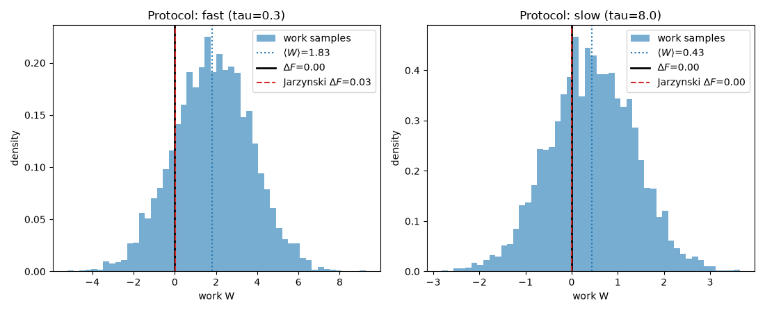
fast (tau=0.3): <W>=1.825, Jarzynski dF_estimate=0.034 (true dF=0)
slow (tau=8.0): <W>=0.433, Jarzynski dF_estimate=0.002 (true dF=0)

Convergence (and bias) of the estimator with ensemble size

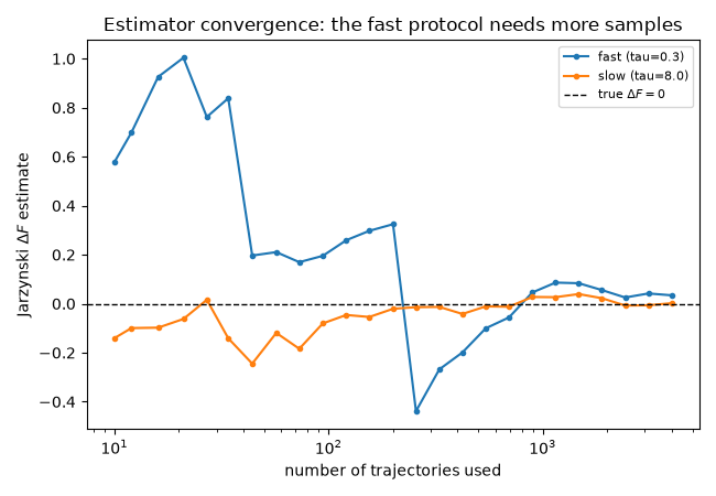
The exponential average defining the Jarzynski estimator is dominated by rare, atypically low-work trajectories, so it is notoriously slow to converge and, for any finite sample, biased high (Jensen’s inequality again, now acting on the estimator itself rather than on <W>). Re-running the same free-energy estimate using only the first n of the 4000 trajectories already generated for each protocol – no new simulation needed – traces out that convergence directly: the faster, more dissipative protocol needs visibly more trajectories to settle near Delta F=0 than the slower, near-reversible one, since a larger spread of work values means the rare low-work trajectories that dominate the average are rarer still.

sample_sizes = np.unique(np.logspace(1, np.log10(4000), 25).astype(int))
plt.figure(figsize=(6.5, 4.5))
for label, (model, work) in work_by_protocol.items():
    running_estimate = [model.jarzynski_free_energy_estimate(work[:n]) for n in sample_sizes]
    plt.plot(sample_sizes, running_estimate, marker="o", ms=3, label=label)
plt.axhline(0.0, color="k", linestyle="--", linewidth=1, label=r"true $\Delta F=0$")
plt.xscale("log")
plt.xlabel("number of trajectories used")
plt.ylabel(r"Jarzynski $\Delta F$ estimate")
plt.title("Estimator convergence: the fast protocol needs more samples")
plt.legend(fontsize=8)
plt.tight_layout()
plt.show()