Path-integral Monte Carlo: a quantum particle as a classical ring polymer

Feynman’s path integral in imaginary time turns the partition function of one quantum particle into that of a classical closed chain of \(P\) beads joined by springs (Barker 1979; Chandler and Wolynes 1981). In units \(\hbar = m = k_B = 1\), with \(\tau = \beta / P\),

\[Z \approx \int dx_1 \cdots dx_P \exp\left[-\sum_j \left(\frac{(x_{j+1}-x_j)^2}{2\tau} + \tau V(x_j)\right)\right],\]

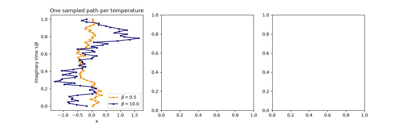
which becomes exact as \(P \to \infty\). Metropolis moves on the beads sample it like any classical system. The spread of the polymer is the quantum delocalization of the particle: at low temperature \(\langle x^2 \rangle\) stays at the zero-point value \(1/(2\omega)\) rather than vanishing as \(1/(\beta\omega^2)\) classically. This example checks the harmonic well against the exact \(\langle x^2 \rangle = \coth(\beta\omega/2)/(2\omega)\), then measures the ground-state energy of the anharmonic well \(V = x^2/2 + x^4\), where no closed form exists.

import matplotlib.pyplot as plt
import numpy as np

from physicskit.statphys.chapters.path_integral import (
    PathIntegralParticle,
    harmonic_x2_exact,
    harmonic_x2_primitive,
)

Ring polymers at high and low temperature

fig, axes = plt.subplots(1, 3, figsize=(13, 4))
for beta, color in [(0.5, "darkorange"), (10.0, "navy")]:
    pimc = PathIntegralParticle(beta, n_beads=64, seed=0)
    pimc.run(n_equil=2000, n_measure=1)
    tau_axis = np.linspace(0.0, beta, 65)
    axes[0].plot(np.append(pimc.path, pimc.path[0]), tau_axis / beta, "o-", ms=3, color=color, label=rf"$\beta = {beta}$")
axes[0].set_xlabel("x")
axes[0].set_ylabel(r"imaginary time $\tau / \beta$")
axes[0].set_title("One sampled path per temperature")
axes[0].legend()

<matplotlib.legend.Legend object at 0x130cdd010>

Harmonic well: the zero-point plateau

betas = np.array([0.25, 0.5, 1.0, 2.0, 4.0, 8.0])
P = 32
x2_mc = []
for b in betas:
    out = PathIntegralParticle(b, n_beads=P, seed=1).run(n_equil=2000, n_measure=40000)
    x2_mc.append(out["x2"])
x2_mc = np.array(x2_mc)
bb = np.geomspace(0.2, 10.0, 200)
axes[1].loglog(bb, harmonic_x2_exact(bb), "k-", label=r"exact $\coth(\beta\omega/2)/2\omega$")
axes[1].loglog(bb, 1.0 / bb, "k:", label=r"classical $1/\beta\omega^2$")
axes[1].loglog(betas, x2_mc, "o", color="crimson", label=f"PIMC, P={P}")
axes[1].axhline(0.5, color="gray", ls="--", lw=0.8)
axes[1].set_xlabel(r"$\beta$")
axes[1].set_ylabel(r"$\langle x^2 \rangle$")
axes[1].set_title("Harmonic oscillator")
axes[1].legend(fontsize=8)
for b, x2 in zip(betas, x2_mc):
    print(f"beta={b:5.2f}: PIMC <x^2> = {x2:.4f}, P={P} exact = {harmonic_x2_primitive(b, P):.4f}, P->inf = {harmonic_x2_exact(b):.4f}")

beta= 0.25: PIMC <x^2> = 4.0247, P=32 exact = 4.0208, P->inf = 4.0208
beta= 0.50: PIMC <x^2> = 2.0269, P=32 exact = 2.0415, P->inf = 2.0415
beta= 1.00: PIMC <x^2> = 1.0965, P=32 exact = 1.0819, P->inf = 1.0820
beta= 2.00: PIMC <x^2> = 0.6639, P=32 exact = 0.6563, P->inf = 0.6565
beta= 4.00: PIMC <x^2> = 0.5249, P=32 exact = 0.5177, P->inf = 0.5187
beta= 8.00: PIMC <x^2> = 0.4912, P=32 exact = 0.4965, P->inf = 0.5003

Anharmonic well: converging the Trotter error

The primitive action has an \(O(\tau^2)\) error, so the virial energy at fixed \(\beta = 10\) (essentially the ground state) is extrapolated linearly in \(1/P^2\) to the continuum limit.

E0_reference = 0.803771  # x^2/2 + x^4, from matrix diagonalization
beads = np.array([16, 32, 64, 128])
E_mc = np.array([PathIntegralParticle(10.0, n_beads=p, lam=1.0, seed=2).run(2000, 60000)["energy"] for p in beads])
slope, E0_extrapolated = np.polyfit(1.0 / beads**2, E_mc, 1)
x = np.linspace(0.0, 1.0 / beads[0] ** 2, 50)
axes[2].plot(1.0 / beads**2, E_mc, "o", color="crimson", label="PIMC virial energy")
axes[2].plot(x, slope * x + E0_extrapolated, "--", color="crimson", lw=1)
axes[2].axhline(E0_reference, color="k", label=f"$E_0 = {E0_reference}$")
axes[2].set_xlabel(r"$1/P^2$")
axes[2].set_ylabel("E")
axes[2].set_title(rf"$V = x^2/2 + x^4$, $\beta = 10$: $E_0 \approx {E0_extrapolated:.3f}$")
axes[2].legend(fontsize=8)
plt.tight_layout()
plt.show()

Check

PIMC reproduces the exact harmonic \(\langle x^2 \rangle\) of the discretized polymer, and the extrapolated anharmonic ground-state energy.

np.testing.assert_allclose(x2_mc, [harmonic_x2_primitive(b, P) for b in betas], rtol=0.06)
assert abs(E0_extrapolated - E0_reference) < 0.02