First- versus second-order transitions in the q-state Potts model

The Potts model generalizes the Ising model (\(q=2\)) to \(q\) discrete states per site: each site of a periodic \(L \times L\) lattice carries a state \(s_i \in \{0, \ldots, q-1\}\), and the Hamiltonian rewards neighboring sites for matching,

\[H = -J \sum_{\langle i,j \rangle} \delta(s_i, s_j),\]

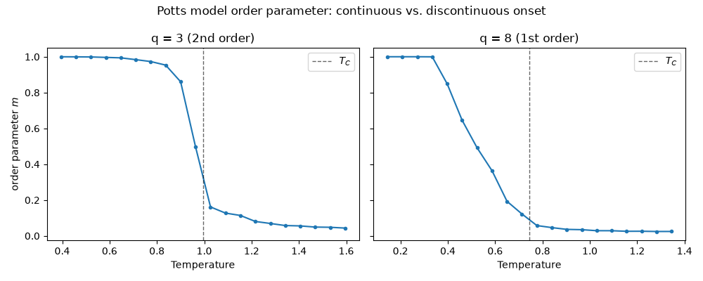
where \(\delta\) is the Kronecker delta. On the square lattice, the Baxter exact solution predicts that the transition, at the exact critical temperature \(T_C = J / (k_B \ln(1+\sqrt{q}))\), stays second order (continuous) for \(q \le 4\) but becomes first order (discontinuous) for \(q > 4\) – the order parameter jumps abruptly rather than vanishing smoothly. This example compares \(q=3\) (second order) against \(q=8\) (first order) by sweeping temperature through each model’s \(T_C\).

import matplotlib.pyplot as plt
import numpy as np

from physicskit.statphys.chapters.ising_lattice import PottsModel2D

Sweep both models across their respective critical points

fig, axes = plt.subplots(1, 2, figsize=(10, 4), sharey=True)

for ax, q in zip(axes, [3, 8]):
    model = PottsModel2D(L=32, q=q, J=1.0, kB=1.0, seed=0)
    temperatures = np.linspace(model.T_C + 0.6, max(model.T_C - 0.6, 0.05), 20)
    result = model.run_temperature_sweep(temperatures, n_equil=150, n_measure=200)

    ax.plot(result["T"], result["m"], marker="o", ms=3)
    ax.axvline(model.T_C, color="k", linestyle="--", linewidth=1, alpha=0.6, label="$T_C$")
    ax.set_xlabel("Temperature")
    ax.set_title(f"q = {q} ({'2nd' if q <= 4 else '1st'} order)")
    ax.legend()

axes[0].set_ylabel("order parameter $m$")
plt.suptitle("Potts model order parameter: continuous vs. discontinuous onset")
plt.tight_layout()

Energy histograms at T_C: the microscopic fingerprint of the order

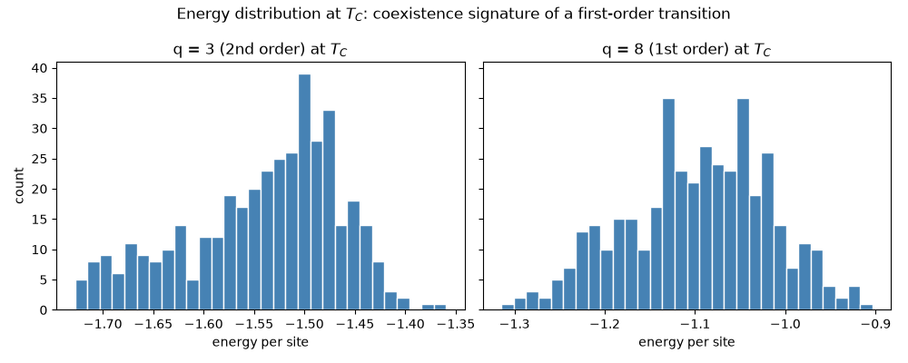
A first-order transition means the ordered and disordered phases coexist at T_C with a nonzero latent heat between them, so a system held exactly at T_C spends time in both phases and its energy histogram is bimodal (two peaks separated by a gap, one per phase). A continuous transition has no latent heat and no phase coexistence, so its energy histogram at T_C stays a single, unimodal peak. Sampling many energies at each model’s own T_C makes this qualitative distinction directly visible.

fig, axes = plt.subplots(1, 2, figsize=(10, 4), sharey=True)
for ax, q in zip(axes, [3, 8]):
    model = PottsModel2D(L=32, q=q, J=1.0, kB=1.0, seed=1)
    beta_c = 1.0 / model.T_C
    model.sweep(beta_c, n_sweeps=300)  # equilibrate at T_C
    energies = np.empty(400)
    for i in range(400):
        model.sweep(beta_c, n_sweeps=5)
        energies[i] = model.energy() / model.n_sites
    ax.hist(energies, bins=30, color="steelblue", edgecolor="white")
    ax.set_xlabel("energy per site")
    ax.set_title(f"q = {q} ({'2nd order' if q <= 4 else '1st order'}) at $T_C$")
axes[0].set_ylabel("count")
plt.suptitle("Energy distribution at $T_C$: coexistence signature of a first-order transition")
plt.tight_layout()
plt.show()