Quantum statistics: Bose-Einstein, Fermi-Dirac, and condensation

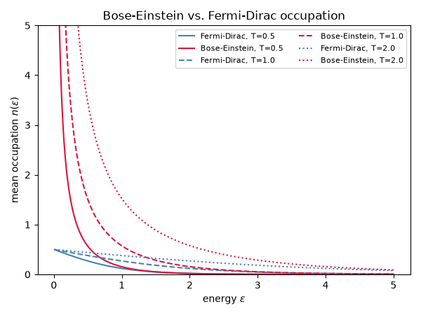
Classical Maxwell-Boltzmann statistics assumes particles are distinguishable and unrestricted in how they can share states. Quantum mechanics changes this in two opposite ways depending on particle spin. Bosons (integer spin) obey the Bose-Einstein distribution

\[n_{\text{BE}}(\varepsilon) = \frac{1}{e^{(\varepsilon-\mu)/k_B T} - 1},\]

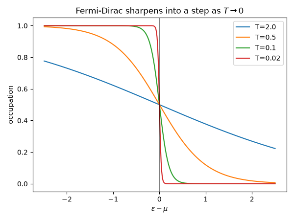
which places no limit on how many particles can pile into the same state, favoring macroscopic occupation of the lowest-energy state at low temperature – Bose-Einstein condensation. Fermions (half-integer spin) instead obey the Pauli exclusion principle via the Fermi-Dirac distribution

\[n_{\text{FD}}(\varepsilon) = \frac{1}{e^{(\varepsilon-\mu)/k_B T} + 1},\]

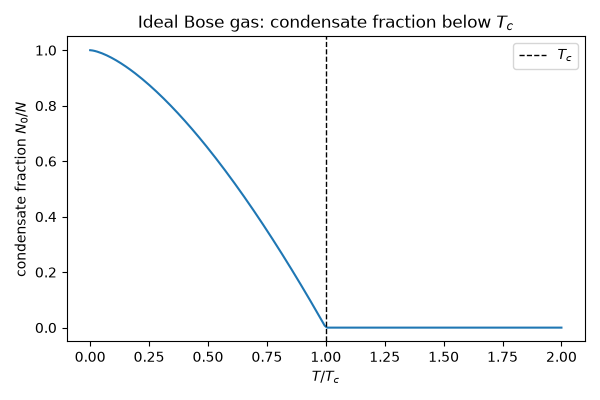
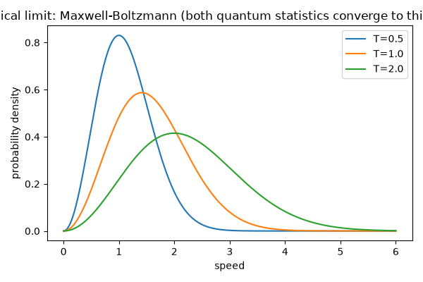
which caps every state’s occupation at 1 and produces a sharp Fermi surface as \(T \to 0\). This example compares all three distributions – \(n_{\text{BE}}\), \(n_{\text{FD}}\), and the classical Maxwell-Boltzmann speed distribution to which both reduce at high temperature – and shows the predicted BEC condensate fraction, first confirmed experimentally in 1995.

import matplotlib.pyplot as plt
import numpy as np

from physicskit.statphys.utils.thermodynamics import (
    bec_condensate_fraction,
    bose_einstein_occupation,
    fermi_dirac_occupation,
    maxwell_boltzmann_speed_pdf,
)

Occupation number versus energy for all three statistics

energy = np.linspace(0.01, 5.0, 400)
mu = 0.0  # chemical potential; Bose-Einstein requires energy > mu everywhere

fig, ax = plt.subplots(figsize=(6, 4.5))
for T, style in zip([0.5, 1.0, 2.0], ["-", "--", ":"]):
    ax.plot(
        energy,
        fermi_dirac_occupation(energy, mu, T),
        style,
        color="steelblue",
        label=f"Fermi-Dirac, T={T}",
    )
    ax.plot(
        energy,
        bose_einstein_occupation(energy, mu - 0.01, T),
        style,
        color="crimson",
        label=f"Bose-Einstein, T={T}",
    )
ax.set_ylim(0, 5)
ax.set_xlabel("energy $\\varepsilon$")
ax.set_ylabel("mean occupation $n(\\varepsilon)$")
ax.legend(fontsize=8, ncol=2)
ax.set_title("Bose-Einstein vs. Fermi-Dirac occupation")
plt.tight_layout()

The Fermi-Dirac step function sharpens as T -> 0

fig, ax = plt.subplots(figsize=(6, 4.5))
for T in [2.0, 0.5, 0.1, 0.02]:
    ax.plot(energy - 2.5, fermi_dirac_occupation(energy, mu=2.5, temperature=T), label=f"T={T}")
ax.axvline(0.0, color="k", linewidth=1, alpha=0.5)
ax.set_xlabel(r"$\varepsilon - \mu$")
ax.set_ylabel("occupation")
ax.legend()
ax.set_title("Fermi-Dirac sharpens into a step as $T \\to 0$")
plt.tight_layout()

Bose-Einstein condensate fraction

T = np.linspace(0.0, 2.0, 200)
fraction = bec_condensate_fraction(T, critical_temperature=1.0)

plt.figure(figsize=(6, 4))
plt.plot(T, fraction)
plt.axvline(1.0, color="k", linestyle="--", linewidth=1, label="$T_c$")
plt.xlabel("$T / T_c$")
plt.ylabel("condensate fraction $N_0/N$")
plt.title("Ideal Bose gas: condensate fraction below $T_c$")
plt.legend()
plt.tight_layout()

For comparison: the classical Maxwell-Boltzmann speed distribution

v = np.linspace(0, 6, 300)
plt.figure(figsize=(6, 4))
for T in [0.5, 1.0, 2.0]:
    plt.plot(v, maxwell_boltzmann_speed_pdf(v, temperature=T, dim=3), label=f"T={T}")
plt.xlabel("speed")
plt.ylabel("probability density")
plt.title("Classical limit: Maxwell-Boltzmann (both quantum statistics converge to this at high T)")
plt.legend()
plt.tight_layout()

The full occupation surface over energy and temperature

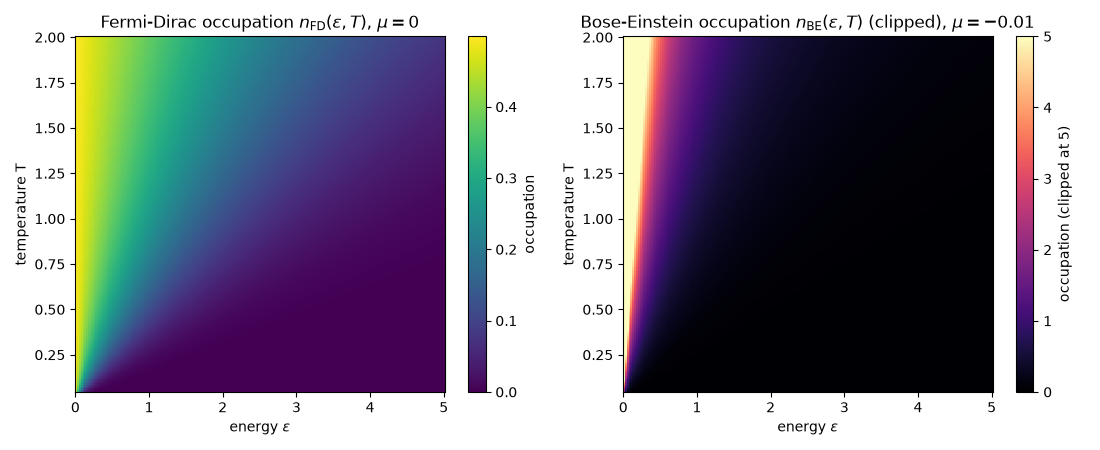
The line plots above only ever show a handful of fixed-T slices through n(energy, T). Evaluating both occupation functions on a full 2D (energy, temperature) grid and rendering them as heatmaps shows the same two functions as continuous surfaces: the Fermi-Dirac heatmap has a sharp occupied/empty boundary that steepens (into a true step) as T -> 0, while the Bose-Einstein heatmap instead blows up along the entire mu=0 edge as T -> 0, reflecting bosons’ unlimited pileup into the lowest state rather than fermions’ one-per-state exclusion.

energy_grid = np.linspace(0.01, 5.0, 200)
T_grid = np.linspace(0.05, 2.0, 200)
E_mesh, T_mesh = np.meshgrid(energy_grid, T_grid)

fd_surface = fermi_dirac_occupation(E_mesh, mu=0.0, temperature=T_mesh)
be_surface = np.clip(bose_einstein_occupation(E_mesh, mu=-0.01, temperature=T_mesh), 0, 5)

fig, axes = plt.subplots(1, 2, figsize=(11, 4.5))
im0 = axes[0].pcolormesh(energy_grid, T_grid, fd_surface, shading="auto", cmap="viridis")
axes[0].set_xlabel(r"energy $\varepsilon$")
axes[0].set_ylabel("temperature T")
axes[0].set_title(r"Fermi-Dirac occupation $n_{\mathrm{FD}}(\varepsilon, T)$, $\mu=0$")
plt.colorbar(im0, ax=axes[0], label="occupation")

im1 = axes[1].pcolormesh(energy_grid, T_grid, be_surface, shading="auto", cmap="magma")
axes[1].set_xlabel(r"energy $\varepsilon$")
axes[1].set_ylabel("temperature T")
axes[1].set_title(r"Bose-Einstein occupation $n_{\mathrm{BE}}(\varepsilon, T)$ (clipped), $\mu=-0.01$")
plt.colorbar(im1, ax=axes[1], label="occupation (clipped at 5)")
plt.tight_layout()
plt.show()