Self-organized criticality: the Bak-Tang-Wiesenfeld sandpile

Ordinary critical phenomena (the Ising transition, percolation) require tuning a parameter – temperature, occupation probability – to a precise critical value. Bak, Tang, and Wiesenfeld’s 1987 sandpile model showed that some driven, dissipative systems tune themselves to criticality through their own dynamics, with no external parameter to adjust.

Grains are dropped one at a time onto a random site of an \(L \times L\) grid with open (absorbing) boundaries. Whenever a site’s height \(z_{i,j}\) reaches the toppling threshold \(z_c\) (4 on the square lattice – one grain per orthogonal neighbor), it topples according to the fixed rule

\[z_{i,j} \to z_{i,j} - z_c, \qquad z_{i\pm1,\,j} \to z_{i\pm1,\,j} + 1, \qquad z_{i,\,j\pm1} \to z_{i,\,j\pm1} + 1,\]

with any grain toppled off the edge of the grid permanently lost. A single toppling can push a neighboring site over threshold too, triggering a cascade – an avalanche – before the pile returns to a stable configuration (\(z_{i,j} < z_c\) everywhere). Slowly adding grains and letting fast avalanches relax the pile drives it, on its own, to a statistically stationary critical state whose avalanche sizes \(s\) follow a power law \(P(s) \sim s^{-\tau}\) with no characteristic scale – this “self-organized criticality” was proposed as a generic mechanism behind the ubiquity of power laws in nature, from earthquakes to solar flares.

import matplotlib.pyplot as plt

from physicskit.statphys.chapters.sandpile import BTWSandpile
from physicskit.statphys.utils.finite_size_scaling import power_law_exponent
from physicskit.statphys.visualizers.sandpile_render import (
    plot_avalanche_size_distribution,
    plot_sandpile_heights,
)

Drive the pile to its self-organized critical state

A \(60 \times 60\) pile is driven with a long warmup (20000 grains, discarded) so it reaches the stationary critical state before 20000 further grains are dropped and each avalanche size recorded. The left panel shows a snapshot of the height field \(z_{i,j} \in \{0, 1, 2, 3\}\); the right panel shows the avalanche-size distribution on log-log axes, whose straight-line shape is the power-law signature of self-organized criticality.

pile = BTWSandpile(L=60, seed=0)
sizes = pile.run(n_grains=20000, warmup=20000)

fig, axes = plt.subplots(1, 2, figsize=(11, 4.5))
plot_sandpile_heights(pile, ax=axes[0])
plot_avalanche_size_distribution(sizes, ax=axes[1])
plt.tight_layout()

print(f"Mean avalanche size: {sizes.mean():.2f}, largest avalanche: {sizes.max()}")

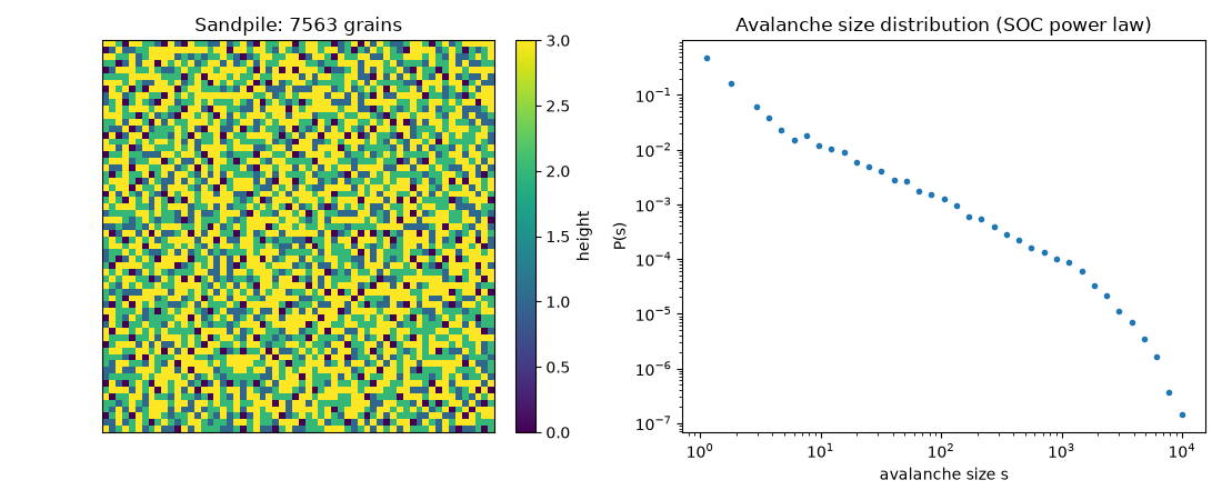
Mean avalanche size: 135.22, largest avalanche: 11184

Finite-size scaling: the cutoff grows with L

The straight-line power law above cannot extend forever: a finite grid caps the largest possible avalanche near its own area, so the distribution actually has a size-dependent cutoff around \(s_{\max} \sim L^{D}\). Running the same self-organizing dynamics at several grid sizes and overlaying their avalanche-size distributions shows the straight-line region growing systematically further to the right (and the largest observed avalanche growing correspondingly) as L increases – the same finite-size-scaling logic used throughout this gallery for thermal critical points, applied here to a self-organized one.

L_values = [20, 40, 60, 90]
max_sizes = []
fig, ax = plt.subplots(figsize=(6.5, 5))
for L in L_values:
    fss_pile = BTWSandpile(L=L, seed=0)
    fss_sizes = fss_pile.run(n_grains=8000, warmup=8 * L * L)
    plot_avalanche_size_distribution(fss_sizes, ax=ax, bins=30)
    max_sizes.append(fss_sizes.max())
# plot_avalanche_size_distribution overwrites the title and labels on every
# call; restore a legend distinguishing the four overlaid curves by color.
for line, L in zip(ax.lines, L_values):
    line.set_label(f"L={L}")
ax.set_title("Avalanche-size cutoff grows with system size L")
ax.legend(fontsize=8)
plt.tight_layout()
plt.show()

cutoff_exponent, _ = power_law_exponent(L_values, max_sizes)
print(f"Largest avalanche by L: {dict(zip(L_values, max_sizes))}")
print(f"Fitted cutoff-growth exponent (max size ~ L^D): D = {cutoff_exponent:.2f} (open-boundary BTW theory: D=2)")

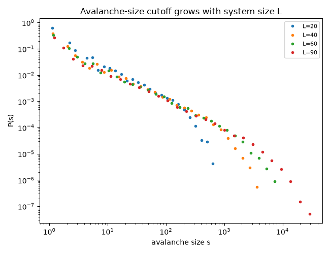
Largest avalanche by L: {20: np.int64(713), 40: np.int64(4213), 60: np.int64(8485), 90: np.int64(50773)}
Fitted cutoff-growth exponent (max size ~ L^D): D = 2.71 (open-boundary BTW theory: D=2)