The Sherrington-Kirkpatrick model and Parisi’s replica overlap

Where the Edwards-Anderson model puts random +/-J bonds on a lattice, the Sherrington-Kirkpatrick (SK) model in 1975 went to the opposite extreme: every spin couples to every other spin, with independent Gaussian bonds

\[H = -\sum_{i<j} J_{ij}\, s_i s_j, \qquad J_{ij} \sim \mathcal{N}\!\left(0, \frac{J^2}{N}\right).\]

The model’s mean-field solution turned out to be far subtler than anyone expected: the naive “replica trick” ansatz gave a negative entropy at low temperature, a clear sign something was wrong, until Giorgio Parisi’s 1979-1980 replica-symmetry-breaking solution revealed that the low- temperature phase is not one frozen state but an infinite, hierarchically organized family of them. The numerically observable fingerprint of this structure is the distribution of the replica overlap

\[q = \frac{1}{N}\sum_i s_i^{(1)} s_i^{(2)}\]

between two independently thermalized replicas sharing the same disorder, pooled across many independent disorder realizations. Above the transition, \(P(q)\) is a single narrow peak at \(q=0\) (replica-symmetric, self-averaging). Below it, finite-size simulations already show a much broader, flatter, non-Gaussian \(P(q)\) – the finite-\(N\) shadow of the continuous distribution Parisi’s solution predicts exactly as \(N \to \infty\).

import matplotlib.pyplot as plt
import numpy as np

from physicskit.statphys.chapters.spin_glass import SherringtonKirkpatrick
from physicskit.statphys.visualizers.spin_glass_render import plot_overlap_distribution

High temperature: a single peak at q = 0

Well above the spin-glass transition (\(T_{SG} \approx J/k_B\) for the SK model), the two replicas decorrelate completely and the pooled overlap distribution is a single narrow peak centered on zero.

model_hot = SherringtonKirkpatrick(N=64, J=1.0, seed=0)
samples_hot = model_hot.overlap_distribution(beta=0.3, n_disorder=25, n_equil=300, n_measure=60)

Low temperature: a broad, structured P(q)

Below the transition, a fresh model instance (a new disorder realization for its first sample) is thermalized at much lower temperature. The resulting pooled distribution is visibly broader and no longer a single peak – finite-size Monte Carlo’s glimpse of replica symmetry breaking.

model_cold = SherringtonKirkpatrick(N=64, J=1.0, seed=1)
samples_cold = model_cold.overlap_distribution(beta=2.0, n_disorder=25, n_equil=300, n_measure=60)

fig, ax = plt.subplots(figsize=(6, 4))
plot_overlap_distribution(samples_hot, ax=ax, label=r"$T=3.3\,J/k_B$ (paramagnetic)")
plot_overlap_distribution(samples_cold, ax=ax, label=r"$T=0.5\,J/k_B$ (spin-glass)")
ax.set_title("Sherrington-Kirkpatrick replica overlap distribution")
plt.tight_layout()
plt.show()

print(f"High-T: mean|q|={abs(samples_hot).mean():.3f}, std(q)={samples_hot.std():.3f}")
print(f"Low-T:  mean|q|={abs(samples_cold).mean():.3f}, std(q)={samples_cold.std():.3f}")

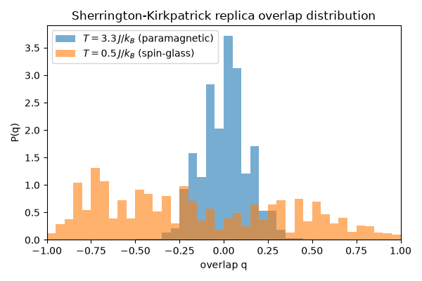
High-T: mean|q|=0.105, std(q)=0.132
Low-T:  mean|q|=0.472, std(q)=0.512

Mean overlap across a full temperature sweep

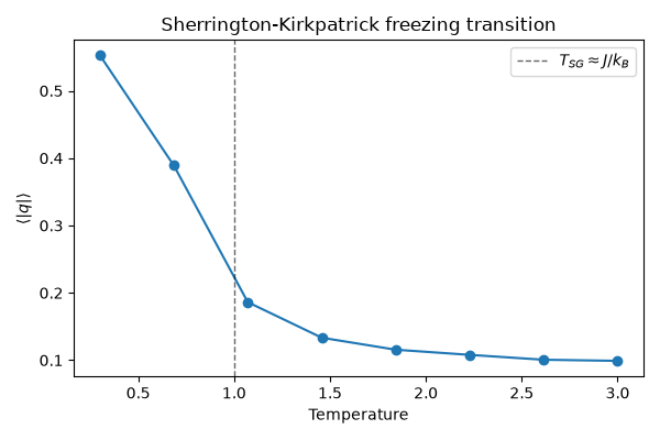
Rather than just the two endpoints above, sweeping \(\langle |q| \rangle\) continuously through \(T_{SG} \approx J/k_B\) shows the freezing transition directly: \(\langle |q| \rangle\) stays near zero in the paramagnetic phase and rises sharply as \(T\) drops below \(T_{SG}\), the SK analogue of the Edwards-Anderson order parameter curve, but built from the same pooled-disorder machinery used above.

T_values = np.linspace(0.3, 3.0, 8)
mean_abs_q = []
for T in T_values:
    model_T = SherringtonKirkpatrick(N=64, J=1.0, seed=2)
    samples_T = model_T.overlap_distribution(beta=1.0 / T, n_disorder=15, n_equil=200, n_measure=40)
    mean_abs_q.append(np.mean(np.abs(samples_T)))

plt.figure(figsize=(6, 4))
plt.plot(T_values, mean_abs_q, marker="o")
plt.axvline(1.0, color="k", linestyle="--", linewidth=1, alpha=0.6, label=r"$T_{SG} \approx J/k_B$")
plt.xlabel("Temperature")
plt.ylabel(r"$\langle |q| \rangle$")
plt.title("Sherrington-Kirkpatrick freezing transition")
plt.legend()
plt.tight_layout()
plt.show()