Wang-Landau sampling of the Ising density of states

Wang and Landau (2001) replaced sampling at a fixed temperature by a random walk in energy. A spin flip from \(E_1\) to \(E_2\) is accepted with probability \(\min(1, g(E_1)/g(E_2))\), and every visit raises the current estimate \(\ln g(E) \to \ln g(E) + \ln f\). The walk is pushed toward rarely visited levels until the histogram is flat; then \(\ln f\) is halved and the walk continues. When \(\ln f\) is small, \(g(E)\) is the density of states, and

\[Z(\beta) = \sum_E g(E)\, e^{-\beta E}\]

gives the thermodynamics at every temperature from one run. This example checks the estimate against exact enumeration on a \(4 \times 4\) lattice, then uses one \(L = 16\) run to draw the specific heat across the transition.

import matplotlib.pyplot as plt
import numpy as np
from scipy.special import logsumexp

from physicskit.statphys.chapters.wang_landau import (
    WangLandauIsing,
    canonical_from_density_of_states,
    ising_density_of_states_exact,
)

Small lattice: Wang-Landau against exact enumeration

E4, g4 = ising_density_of_states_exact(4)
wl4 = WangLandauIsing(L=4, seed=0)
_, log_g4 = wl4.run(log_f_final=1e-6)
ok = g4 > 0
max_err = np.max(np.abs(log_g4[ok] - np.log(g4[ok])))
print(f"L=4: max |ln g_WL - ln g_exact| = {max_err:.3f} over {ok.sum()} levels")

fig, axes = plt.subplots(1, 3, figsize=(13, 4))
axes[0].plot(E4[ok] / 16, np.log(g4[ok]), "k-", lw=2, label="exact enumeration")
axes[0].plot(E4[ok] / 16, log_g4[ok], "o", color="crimson", label="Wang-Landau")
axes[0].set_xlabel("E / N")
axes[0].set_ylabel(r"$\ln g(E)$")
axes[0].set_title(r"$4\times4$ lattice")
axes[0].legend()

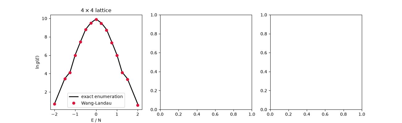
L=4: max |ln g_WL - ln g_exact| = 0.126 over 15 levels

<matplotlib.legend.Legend object at 0x130ccb650>

Larger lattice: one run, every temperature

L = 16
N = L * L
wl = WangLandauIsing(L=L, seed=1)
E, log_g = wl.run(log_f_final=1e-6)
finite = np.isfinite(log_g)
axes[1].plot(E[finite] / N, log_g[finite] / N, color="crimson")
axes[1].set_xlabel("E / N")
axes[1].set_ylabel(r"$\ln g(E) / N$")
axes[1].set_title(rf"$L={L}$: $\ln g$ spans {log_g[finite].max() / np.log(10):.0f} decades")

T = np.linspace(1.2, 4.0, 300)
thermo = canonical_from_density_of_states(E, log_g, T, n_sites=N)
T_peak = T[np.argmax(thermo["C_v"])]
T_C = 2.0 / np.log(1.0 + np.sqrt(2.0))
axes[2].plot(T, thermo["C_v"], color="crimson", label=f"Wang-Landau, L={L}")
axes[2].axvline(T_C, color="gray", ls="--", label=rf"Onsager $T_C = {T_C:.3f}$")
axes[2].set_xlabel("T")
axes[2].set_ylabel(r"$C_v$ per site")
axes[2].set_title(f"Specific heat peak at T = {T_peak:.3f}")
axes[2].legend()
plt.tight_layout()
plt.show()
print(f"modification factor halved {len(wl.log_f_history)} times; C_v peak at T = {T_peak:.3f}")

modification factor halved 20 times; C_v peak at T = 2.324

Check

The 4x4 estimate matches enumeration, the total number of states is \(2^N\), and the specific-heat peak sits within a few percent of Onsager’s \(T_C\) (shifted upward by finite size).

assert max_err < 0.15
assert abs(logsumexp(log_g[finite]) - N * np.log(2.0)) < 0.01 * N * np.log(2.0)
assert abs(T_peak - T_C) / T_C < 0.05