The Lee-Yang circle theorem: partition function zeros in the complex plane

A finite system’s partition function is a finite sum of manifestly analytic terms – so where can a genuine phase transition, a true discontinuity in the free energy, possibly come from? Lee and Yang’s 1952 answer: continue the partition function into the complex fugacity plane and look at its zeros. Writing the Ising Hamiltonian with a field,

\[H = -J\sum_{\langle i,j \rangle} s_i s_j - h \sum_i s_i, \qquad z = e^{2\beta h},\]

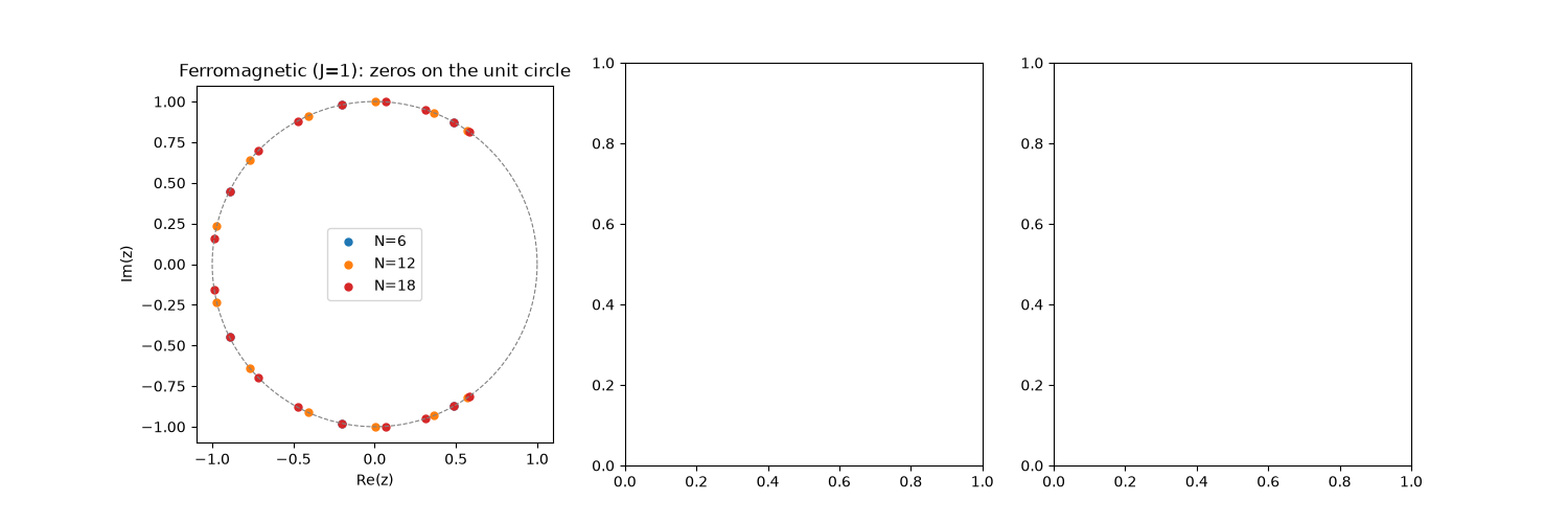
the partition function is (up to a nonvanishing analytic prefactor) a degree-\(N\) polynomial in the fugacity \(z\). Lee and Yang proved that for a ferromagnetic system (\(J > 0\)), every one of that polynomial’s \(N\) roots lies exactly on the unit circle \(|z| = 1\), no matter the system size. A phase transition occurs, in the \(N\to\infty\) limit, exactly where these zeros pinch the positive real axis at \(z=1\) (\(h=0\)); for antiferromagnetic coupling, the theorem simply does not apply, and the zeros scatter off the circle entirely.

import matplotlib.pyplot as plt
import numpy as np

from physicskit.statphys.utils.partition_function import ising_partition_polynomial, yang_lee_zeros

Ferromagnetic zeros: exactly on the unit circle

For J > 0, every zero of Z(z) lands on \(|z|=1\) to machine precision, regardless of chain length – and as N grows, more zeros appear, crowding ever more densely near z=1 (h=0), foreshadowing where the infinite-system free energy will develop its singularity.

fig, axes = plt.subplots(1, 3, figsize=(15, 5))
theta = np.linspace(0, 2 * np.pi, 200)
axes[0].plot(np.cos(theta), np.sin(theta), color="gray", linewidth=0.8, linestyle="--")

for N, color in zip([6, 12, 18], ["tab:blue", "tab:orange", "tab:red"]):
    g = ising_partition_polynomial(N, beta=0.4, J=1.0, periodic=True)
    zeros = yang_lee_zeros(g)
    axes[0].scatter(zeros.real, zeros.imag, s=25, color=color, label=f"N={N}")

axes[0].set_xlabel("Re(z)")
axes[0].set_ylabel("Im(z)")
axes[0].set_title("Ferromagnetic (J=1): zeros on the unit circle")
axes[0].set_aspect("equal")
axes[0].legend()

<matplotlib.legend.Legend object at 0x157309220>

Antiferromagnetic zeros: no such constraint

Flipping the sign of J removes the ferromagnetic hypothesis the circle theorem depends on; the zeros scatter well off the unit circle.

g_af = ising_partition_polynomial(14, beta=0.4, J=-1.0, periodic=True)
zeros_af = yang_lee_zeros(g_af)
axes[1].scatter(zeros_af.real, zeros_af.imag, s=25, color="tab:purple")
axes[1].set_xlabel("Re(z)")
axes[1].set_ylabel("Im(z)")
axes[1].set_title("Antiferromagnetic (J=-1, N=14):\nzeros scattered on the real axis")
axes[1].axhline(0, color="black", linewidth=0.5)
axes[1].text(
    0.03,
    0.94,
    "all 14 zeros are real\n(spanning roughly -18 to 0,\nnot confined to any circle)",
    transform=axes[1].transAxes,
    fontsize=9,
    va="top",
)

# The antiferromagnetic zeros span roughly [-18, 0] on the real axis, so at
# the scale needed to show all of them the |z|=1 reference circle would be
# an invisible speck; a separate, explicitly zoomed panel keeps that
# comparison visible for the several roots that land closest to the origin.
axes[2].plot(np.cos(theta), np.sin(theta), color="gray", linewidth=0.8, linestyle="--")
axes[2].scatter(zeros_af.real, zeros_af.imag, s=25, color="tab:purple")
axes[2].set_xlim(-1.3, 1.3)
axes[2].set_ylim(-1.3, 1.3)
axes[2].set_aspect("equal")
axes[2].set_xlabel("Re(z)")
axes[2].set_ylabel("Im(z)")
axes[2].set_title("Zoom near the origin:\nno zero actually sits on $|z|=1$")

plt.tight_layout()
plt.show()

g_check = ising_partition_polynomial(18, beta=0.4, J=1.0, periodic=True)
z_check = yang_lee_zeros(g_check)
print(f"Ferromagnetic N=18: max deviation from |z|=1 is {np.max(np.abs(np.abs(z_check) - 1)):.2e}")

Ferromagnetic N=18: max deviation from |z|=1 is 6.25e-13