The Karplus relation: vicinal 3J(H,H) coupling as a function of dihedral angle

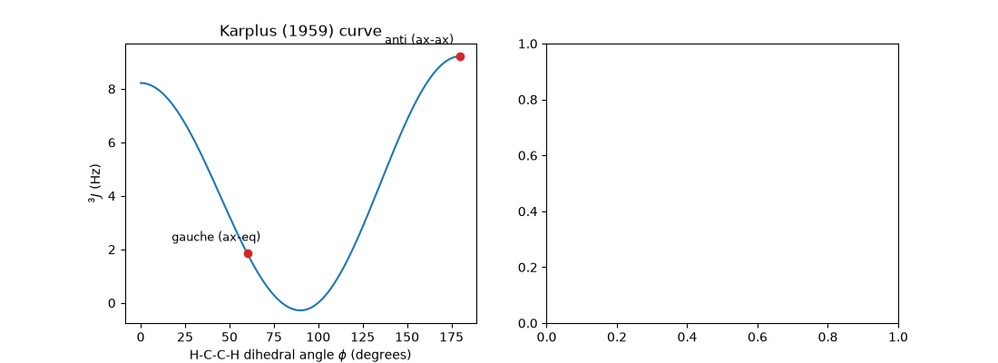
Karplus (1959) used valence-bond theory to show that the three-bond (vicinal) H-C-C-H coupling constant depends on the dihedral angle \(\phi\). It is large for eclipsed (0 degrees) and anti (180 degrees) protons and nearly zero near 90 degrees. This lets a measured \(^3J\) report molecular conformation. This example plots Karplus’s 1959 curve from karplus_coupling(), reads off the axial-axial and axial-equatorial couplings of a cyclohexane chair, and shows the resulting doublet splittings.

import matplotlib.pyplot as plt
import numpy as np

from chemistrykit.spectro.systems.nmr import first_order_multiplet, karplus_coupling
from chemistrykit.spectro.visualizers.spectro_plots import plot_broadened_spectrum

phi = np.linspace(0.0, 180.0, 361)
j_1959 = karplus_coupling(phi)

# In an ideal cyclohexane chair, axial-axial vicinal protons are anti
# (~180 degrees); axial-equatorial and equatorial-equatorial are gauche (~60 degrees).
j_ax_ax = karplus_coupling(180.0)
j_ax_eq = karplus_coupling(60.0)
print(f"3J(axial-axial, 180 deg)  = {j_ax_ax:.2f} Hz")
print(f"3J(axial-equatorial, 60 deg) = {j_ax_eq:.2f} Hz")
print(f"3J at 90 deg = {karplus_coupling(90.0):.2f} Hz (minimum)")

3J(axial-axial, 180 deg)  = 9.22 Hz
3J(axial-equatorial, 60 deg) = 1.85 Hz
3J at 90 deg = -0.28 Hz (minimum)

fig, (ax1, ax2) = plt.subplots(1, 2, figsize=(11, 4))
ax1.plot(phi, j_1959, color="tab:blue")
for angle, label in ((60.0, "gauche (ax-eq)"), (180.0, "anti (ax-ax)")):
    ax1.plot(angle, karplus_coupling(angle), "o", color="tab:red")
    ax1.annotate(label, (angle, karplus_coupling(angle)), xytext=(-60, 10), textcoords="offset points", fontsize=9)
ax1.set_xlabel(r"H-C-C-H dihedral angle $\phi$ (degrees)")
ax1.set_ylabel(r"$^3J$ (Hz)")
ax1.set_title("Karplus (1959) curve")

Text(0.5, 1.0, 'Karplus (1959) curve')

The same proton coupled to one anti neighbour vs. one gauche neighbour: a wide doublet vs. a narrow one.

x = np.linspace(3.45, 3.55, 3000)
wide = first_order_multiplet(chemical_shift_ppm=3.5, j_coupling_hz=j_ax_ax, n_neighbors=1, spectrometer_frequency_mhz=400.0)
narrow = first_order_multiplet(chemical_shift_ppm=3.5, j_coupling_hz=j_ax_eq, n_neighbors=1, spectrometer_frequency_mhz=400.0)
plot_broadened_spectrum(wide, x, ax=ax2, shape="lorentzian", fwhm=0.002, color="tab:red", label=f"anti: J = {j_ax_ax:.1f} Hz")
plot_broadened_spectrum(narrow, x, ax=ax2, shape="lorentzian", fwhm=0.002, color="tab:green", label=f"gauche: J = {j_ax_eq:.1f} Hz")
ax2.invert_xaxis()
ax2.set_xlabel("chemical shift (ppm)")
ax2.set_title("Doublet splitting reports the dihedral angle")
ax2.legend()
fig.tight_layout()
plt.show()