Constable’s compensation effect across a catalyst series

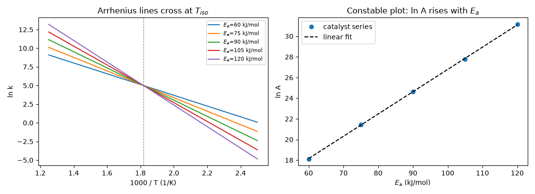
Constable (1925) found that across a series of similar catalysts, a higher activation energy \(E_a\) came with a higher pre-exponential factor \(A\), so \(\ln A\) rose linearly with \(E_a\):

\[\ln A = \alpha + \frac{E_a}{RT_{iso}}.\]

When that holds, every catalyst in the series has the same rate constant at the isokinetic temperature \(T_{iso}\), and their Arrhenius lines all cross there. This example builds such a series and uses compare_catalyzed_rate(), which takes separate \(E_a\) and \(A\) values for the two pathways. It then recovers \(T_{iso}\) from the slope of the Constable plot. The rate enhancement over a reference catalyst is exactly 1 at \(T_{iso}\).

import matplotlib.pyplot as plt
import numpy as np

from chemistrykit.constants import R
from chemistrykit.surface.systems.catalysis import compare_catalyzed_rate

T_iso = 550.0  # K
alpha = 5.0
Ea_series = np.array([60e3, 75e3, 90e3, 105e3, 120e3])
lnA_series = alpha + Ea_series / (R * T_iso)

rng = np.random.default_rng(7)
lnA_measured = lnA_series + rng.normal(scale=0.2, size=Ea_series.shape)
slope, intercept = np.polyfit(Ea_series, lnA_measured, 1)
print(f"True isokinetic temperature:           {T_iso:.1f} K")
print(f"Recovered from the Constable plot:     {1.0 / (R * slope):.1f} K")

True isokinetic temperature:           550.0 K
Recovered from the Constable plot:     557.1 K

Rate enhancement of each catalyst over the lowest-Ea member, above, at, and below T_iso: the ordering flips at T_iso.

ref_Ea, ref_A = Ea_series[0], np.exp(lnA_series[0])
for T in [450.0, T_iso, 650.0]:
    ratios = [compare_catalyzed_rate(ref_Ea, Ea, T, A_uncatalyzed=ref_A, A_catalyzed=np.exp(lnA)).rate_enhancement for Ea, lnA in zip(Ea_series, lnA_series)]
    print(f"T = {T:5.1f} K: k/k_ref = " + ", ".join(f"{r:.3g}" for r in ratios))

T = 450.0 K: k/k_ref = 1, 0.482, 0.233, 0.112, 0.0542
T = 550.0 K: k/k_ref = 1, 1, 1, 1, 1
T = 650.0 K: k/k_ref = 1, 1.66, 2.74, 4.54, 7.53

invT = np.linspace(1 / 800.0, 1 / 400.0, 200)
fig, axes = plt.subplots(1, 2, figsize=(11, 4))
for Ea, lnA in zip(Ea_series, lnA_series):
    axes[0].plot(1e3 * invT, lnA - Ea / R * invT, label=f"$E_a$={Ea / 1e3:.0f} kJ/mol")
axes[0].axvline(1e3 / T_iso, color="gray", linestyle="--", linewidth=0.8)
axes[0].set_xlabel("1000 / T (1/K)")
axes[0].set_ylabel("ln k")
axes[0].set_title("Arrhenius lines cross at $T_{iso}$")
axes[0].legend(fontsize=8)

axes[1].plot(Ea_series / 1e3, lnA_measured, "o", label="catalyst series")
axes[1].plot(Ea_series / 1e3, slope * Ea_series + intercept, "k--", label="linear fit")
axes[1].set_xlabel("$E_a$ (kJ/mol)")
axes[1].set_ylabel("ln A")
axes[1].set_title("Constable plot: ln A rises with $E_a$")
axes[1].legend()
plt.tight_layout()
plt.show()