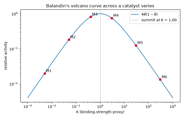
Balandin’s volcano curve: catalytic activity peaks at intermediate binding

Balandin’s multiplet theory (1929) predicted that when catalytic activity is plotted against binding strength across a series of catalysts, it rises, peaks and falls again, tracing a “volcano”. Bligaard, Norskov and coworkers (2004) later derived that shape from the Bronsted-Evans-Polanyi relation. This example reproduces the volcano with the standard textbook toy model (Chorkendorff & Niemantsverdriet, Concepts of Modern Catalysis and Kinetics, 2nd ed., Wiley-VCH, 2007, Ch. 8). The rate needs an occupied site to hold the intermediate and an empty site for the next step, so rate \(\propto\theta(1-\theta)\), with \(\theta\) the Langmuir coverage (langmuir_coverage()). The adsorption constant \(K\) stands in for binding strength. A hypothetical series of catalysts sits on the two legs of the volcano, and its summit is exactly Langmuir’s half-saturation point \(K = 1/P\). This is not a literal reproduction of Balandin’s multiplet equations.

import matplotlib.pyplot as plt
import numpy as np

from chemistrykit.surface.systems.langmuir import LangmuirIsotherm, langmuir_coverage

P = 1.0
K_values = np.logspace(-3, 3, 4000)
theta = langmuir_coverage(K_values, P)
rate = theta * (1.0 - theta)

peak_index = int(np.argmax(rate))
K_peak = K_values[peak_index]
print(f"Rate-maximizing K: {K_peak:.4f} (theory: 1/P = {1.0 / P:.4f})")
print(f"Coverage there: {theta[peak_index]:.4f} (theory: exactly 0.5)")
iso_at_peak = LangmuirIsotherm(K=K_peak, qmax=1.0)
print(f"Half-saturation pressure of the summit catalyst: {iso_at_peak.half_saturation_pressure():.4f} (= P)")

Rate-maximizing K: 0.9983 (theory: 1/P = 1.0000)
Coverage there: 0.4996 (theory: exactly 0.5)
Half-saturation pressure of the summit catalyst: 1.0017 (= P)

A hypothetical catalyst series, from weak to strong binders. Plotted against binding strength, they fall on the two legs of the volcano.

series = {"M1": 0.005, "M2": 0.05, "M3": 0.4, "M4": 3.0, "M5": 30.0, "M6": 300.0}
for name, K in series.items():
    th = langmuir_coverage(K, P)
    leg = "left (too weak)" if K < 1 / P else "right (too strong)"
    print(f"{name}: K = {K:7.3f}, relative activity = {th * (1 - th) / 0.25:.3f}, {leg}")

M1: K =   0.005, relative activity = 0.020, left (too weak)
M2: K =   0.050, relative activity = 0.181, left (too weak)
M3: K =   0.400, relative activity = 0.816, left (too weak)
M4: K =   3.000, relative activity = 0.750, right (too strong)
M5: K =  30.000, relative activity = 0.125, right (too strong)
M6: K = 300.000, relative activity = 0.013, right (too strong)

fig, ax = plt.subplots(figsize=(7, 4.5))
ax.loglog(K_values, rate / 0.25, label=r"$4\theta(1-\theta)$")
for name, K in series.items():
    th = langmuir_coverage(K, P)
    ax.plot(K, th * (1 - th) / 0.25, "o", color="crimson")
    ax.annotate(name, (K, th * (1 - th) / 0.25), textcoords="offset points", xytext=(4, 4))
ax.axvline(K_peak, color="gray", linestyle="--", linewidth=0.8, label=f"summit at K = {K_peak:.2f}")
ax.set_xlabel("K (binding-strength proxy)")
ax.set_ylabel("relative activity")
ax.set_title("Balandin's volcano curve across a catalyst series")
ax.legend()
plt.tight_layout()
plt.show()