Antoine’s equation: vapor pressure beyond Clausius-Clapeyron

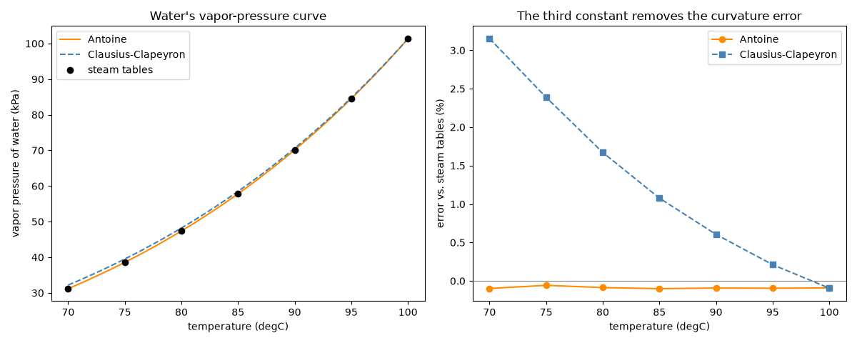
The integrated Clausius-Clapeyron equation assumes a constant enthalpy of vaporization, so \(\ln P\) is exactly linear in \(1/T\). Real vapor-pressure curves bend slightly, because \(\Delta H_{vap}\) shrinks as the temperature rises toward the critical point. Antoine’s three-constant equation (AntoineEquation), \(\log_{10}P = A - B/(C+T)\), absorbs that curvature in the single extra constant \(C\). Below, both are compared with steam-table values for water. The Antoine curve uses the NIST constants for 344-373 K.

import matplotlib.pyplot as plt
import numpy as np

from chemistrykit.thermo import AntoineEquation, ClausiusClapeyron

water = AntoineEquation(A=5.08354, B=1663.125, C=-45.622)  # P in bar, T in K (NIST, 344-373 K)
cc = ClausiusClapeyron(delta_h_vap=40700.0, T_ref=373.15, P_ref=101325.0)

# Saturation pressures of water from the IAPWS steam tables, in kPa.
T_table = np.array([343.15, 348.15, 353.15, 358.15, 363.15, 368.15, 373.15])
P_table = np.array([31.20, 38.58, 47.41, 57.87, 70.18, 84.61, 101.42])

T = np.linspace(343.15, 373.15, 200)
P_antoine = water.pressure(T) * 100.0  # bar -> kPa
P_cc = cc.pressure(T) / 1000.0

fig, axes = plt.subplots(1, 2, figsize=(12, 4.8))
axes[0].plot(T - 273.15, P_antoine, color="darkorange", label="Antoine")
axes[0].plot(T - 273.15, P_cc, "--", color="steelblue", label="Clausius-Clapeyron")
axes[0].plot(T_table - 273.15, P_table, "ko", label="steam tables")
axes[0].set_xlabel("temperature (degC)")
axes[0].set_ylabel("vapor pressure of water (kPa)")
axes[0].set_title("Water's vapor-pressure curve")
axes[0].legend()

err_antoine = 100 * (water.pressure(T_table) * 100.0 - P_table) / P_table
err_cc = 100 * (cc.pressure(T_table) / 1000.0 - P_table) / P_table
axes[1].plot(T_table - 273.15, err_antoine, "o-", color="darkorange", label="Antoine")
axes[1].plot(T_table - 273.15, err_cc, "s--", color="steelblue", label="Clausius-Clapeyron")
axes[1].axhline(0.0, color="gray", linewidth=0.8)
axes[1].set_xlabel("temperature (degC)")
axes[1].set_ylabel("error vs. steam tables (%)")
axes[1].set_title("The third constant removes the curvature error")
axes[1].legend()
fig.tight_layout()

The equation inverts in closed form, giving the boiling point at any pressure – here, water boiling at reduced pressure:

for P_kPa in (101.325, 70.0, 47.0):
    print(f"P = {P_kPa:7.3f} kPa -> T_boil = {float(water.temperature(P_kPa / 100.0)) - 273.15:5.1f} degC")

plt.show()

P = 101.325 kPa -> T_boil = 100.0 degC
P =  70.000 kPa -> T_boil =  90.0 degC
P =  47.000 kPa -> T_boil =  79.8 degC