Oort and Zwicky: missing mass from velocity dispersions

Oort (1932) and Zwicky (1933) both turned observed random velocities into a gravitating mass and found more mass than they could see.

• Oort used the vertical motions of stars near the Sun: stars bouncing through the Galactic disk with dispersion \(\sigma_z\) stay within a scale height \(z_0\) set by the local mass density. For a self-gravitating isothermal sheet, \(\rho(z)=\rho_0\,\mathrm{sech}^2(z/z_0)\) with \(\rho_0=\sigma_z^2/(2\pi G z_0^2)\).

• Zwicky applied the virial theorem, \(2\langle T\rangle + \langle U\rangle = 0\), to the galaxies of the Coma Cluster, giving \(M_{\rm vir}\approx 5\sigma^2R/G\) from the line-of-sight velocity dispersion \(\sigma\) and the cluster radius \(R\).

Both estimates are reproduced here in SI units from physicskit.constants, with illustrative, round-number inputs close to the historical values.

import matplotlib.pyplot as plt
import numpy as np

from physicskit.constants import PARSEC_M, SOLAR_MASS_KG, G

KM = 1e3
MSUN_PER_PC3 = SOLAR_MASS_KG / PARSEC_M**3

Oort (1932): the local density from vertical star motions

A sample of disk stars with a vertical velocity dispersion of \(\sigma_z\approx 20\) km/s, confined to a sheet with scale height \(z_0\approx 350\) pc, requires a mid-plane density near \(0.12\,M_\odot/{\rm pc}^3\) – more than the stars and gas Oort could count at the time.

sigma_z = 20.0 * KM
z0 = 350.0 * PARSEC_M
rho0 = sigma_z**2 / (2.0 * np.pi * G * z0**2)
rho_visible = 0.08 * MSUN_PER_PC3  # stars + gas counted locally (illustrative)
print(f"Oort: dynamical mid-plane density  = {rho0 / MSUN_PER_PC3:.3f} Msun/pc^3")
print(f"      visible (counted) density    = {rho_visible / MSUN_PER_PC3:.3f} Msun/pc^3")
print(f"      dynamical / visible          = {rho0 / rho_visible:.2f}")

z_pc = np.linspace(-1500, 1500, 400)
fig1, ax1 = plt.subplots(figsize=(5.5, 3.8))
ax1.plot(z_pc, rho0 / MSUN_PER_PC3 / np.cosh(z_pc * PARSEC_M / z0) ** 2, color="steelblue", label=r"required by $\sigma_z$")
ax1.plot(z_pc, rho_visible / MSUN_PER_PC3 / np.cosh(z_pc * PARSEC_M / z0) ** 2, "--", color="firebrick", label="visible stars + gas")
ax1.set_xlabel("height above the Galactic plane $z$ [pc]")
ax1.set_ylabel(r"$\rho(z)$ [$M_\odot$/pc$^3$]")
ax1.set_title("Oort: the isothermal-sheet density")
ax1.legend(fontsize=8)
fig1.tight_layout()

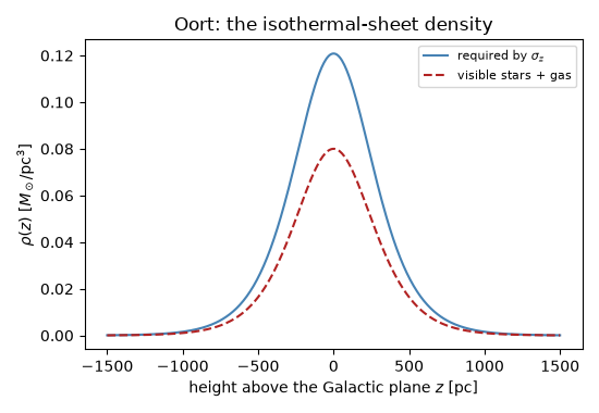
Oort: dynamical mid-plane density  = 0.121 Msun/pc^3
      visible (counted) density    = 0.080 Msun/pc^3
      dynamical / visible          = 1.51

Zwicky (1933): the virial mass of the Coma Cluster

Draw 800 member galaxies with a mean recession velocity of 6900 km/s and a line-of-sight dispersion of 1000 km/s, as a redshift survey would see them. The sample dispersion alone, with a radius of 1 Mpc, fixes the virial mass; bootstrapping the sample gives its statistical spread.

rng = np.random.default_rng(1933)
v_los = rng.normal(6900.0, 1000.0, size=800)  # km/s
R = 1.0e6 * PARSEC_M


def virial_mass(v_kms):
    sigma = np.std(v_kms, ddof=1) * KM
    return 5.0 * sigma**2 * R / G / SOLAR_MASS_KG


M_vir = virial_mass(v_los)
M_boot = np.array([virial_mass(rng.choice(v_los, v_los.size)) for _ in range(500)])

L_cluster = 5e12  # total luminosity in solar units (illustrative)
M_over_L_stars = 3.0
M_luminous = M_over_L_stars * L_cluster
print(f"\nZwicky: sample sigma_los       = {np.std(v_los, ddof=1):.0f} km/s")
print(f"        virial mass              = {M_vir:.2e} Msun  (bootstrap +/- {M_boot.std():.1e})")
print(f"        luminous mass (M/L = 3)  = {M_luminous:.2e} Msun")
print(f"        virial / luminous        = {M_vir / M_luminous:.0f}  (Zwicky's 'dunkle Materie')")

fig2, (ax2, ax3) = plt.subplots(1, 2, figsize=(10, 3.8))
ax2.hist(v_los, bins=40, color="steelblue", alpha=0.8)
ax2.set_xlabel("line-of-sight velocity [km/s]")
ax2.set_ylabel("galaxies")
ax2.set_title("Coma-like cluster: redshift velocities")
ax3.hist(M_boot, bins=30, color="darkorchid", alpha=0.8, label="virial mass (bootstrap)")
ax3.axvline(M_luminous, color="firebrick", ls="--", label="luminous mass")
ax3.set_xscale("log")
ax3.set_xlim(M_luminous / 3, M_vir * 3)
ax3.set_xlabel(r"mass [$M_\odot$]")
ax3.set_title("Zwicky: virial mass vs. starlight")
ax3.legend(fontsize=8)
fig2.tight_layout()

plt.show()

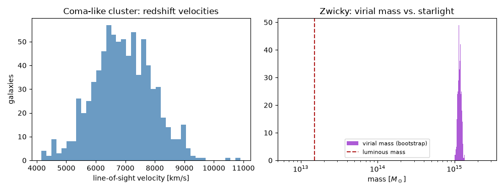
Zwicky: sample sigma_los       = 1004 km/s
        virial mass              = 1.17e+15 Msun  (bootstrap +/- 6.1e+13)
        luminous mass (M/L = 3)  = 1.50e+13 Msun
        virial / luminous        = 78  (Zwicky's 'dunkle Materie')

Check

Oort’s sheet needs more mass than is seen; Zwicky’s virial mass 5 sigma^2 R / G (sigma ~ 1000 km/s, R = 1 Mpc) is ~1.2e15 Msun, tens of times the starlight.

assert rho0 / rho_visible > 1.2
assert abs(M_vir - 5 * (1000 * KM) ** 2 * R / G / SOLAR_MASS_KG) < 3 * M_boot.std() + 0.02 * M_vir
assert M_vir / M_luminous > 30