Rubin and Ford: flat galaxy rotation curves

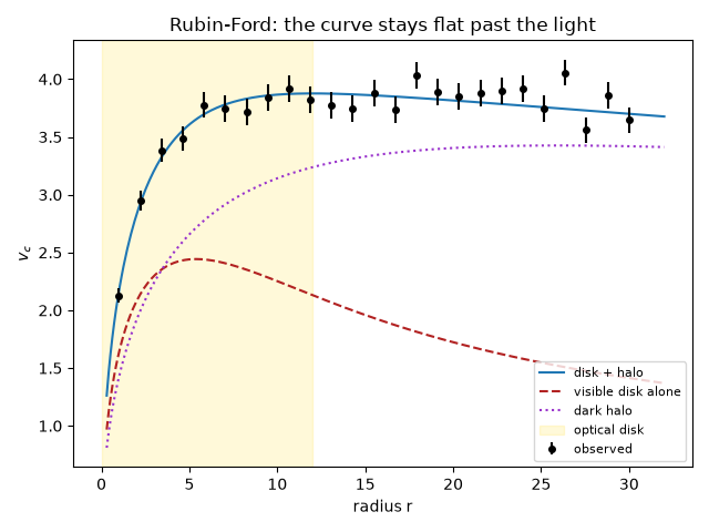
Rubin and Ford (1970) measured the Doppler shifts of emission regions across the Andromeda galaxy, and through the 1970s they, Roberts, Whitehurst and Bosma extended such curves far past the visible disk. If the visible stars and gas were all the mass, the circular speed \(v_c(r)=\sqrt{GM(<r)/r}\) would fall as \(r^{-1/2}\) once the light runs out. Instead it stays flat.

This example builds a mock observed rotation curve, compares it with the visible disk alone using circular_velocity(), and shows that the outer points require an extended halo, here an NFW halo from nfw_enclosed_mass(). Units are \(G=1\).

import matplotlib.pyplot as plt
import numpy as np

from physicskit.astro.galactic_dynamics import circular_velocity, nfw_enclosed_mass
from physicskit.astro.visualizers import plot_rotation_curve

Visible matter: an exponential disk

Surface brightness falls off as \(e^{-r/R_d}\). In the spherical approximation its enclosed mass is \(M_d[1-(1+r/R_d)e^{-r/R_d}]\), which saturates at \(M_d\) beyond a few scale lengths.

M_disk, R_d = 60.0, 3.0


def disk_mass(r):
    x = np.asarray(r, dtype=float) / R_d
    return M_disk * (1.0 - (1.0 + x) * np.exp(-x))


rho_s, r_s = 0.03, 12.0


def total_mass(r):
    return disk_mass(r) + nfw_enclosed_mass(r, rho_s, r_s)

Mock observations

Twenty-five emission regions and 21-cm points, out to ten disk scale lengths, with a 3% velocity error each. The “true” galaxy is disk plus halo; the observer does not know that.

rng = np.random.default_rng(1970)
r_obs = np.linspace(1.0, 30.0, 25)
v_true = circular_velocity(r_obs, total_mass)
v_err = 0.03 * v_true
v_obs = v_true + rng.normal(0.0, v_err)

r = np.linspace(0.3, 32.0, 300)
v_disk = circular_velocity(r, disk_mass)
v_halo = circular_velocity(r, lambda x: nfw_enclosed_mass(x, rho_s, r_s))
v_model = circular_velocity(r, total_mass)

fig1, ax1 = plot_rotation_curve(r, v_model, v_observed=None)
ax1.lines[0].set_label("disk + halo")
ax1.errorbar(r_obs, v_obs, yerr=v_err, fmt="o", color="black", ms=4, label="observed")
ax1.plot(r, v_disk, "--", color="firebrick", label="visible disk alone")
ax1.plot(r, v_halo, ":", color="darkorchid", label="dark halo")
ax1.axvspan(0, 4 * R_d, color="gold", alpha=0.15, label="optical disk")
ax1.set_xlabel("radius r")
ax1.set_ylabel(r"$v_c$")
ax1.set_title("Rubin-Ford: the curve stays flat past the light")
ax1.legend(fontsize=8, loc="lower right")
fig1.tight_layout()

The mass discrepancy grows with radius

Inverting \(v_c^2=GM/r\) turns each observed speed into a dynamical mass. A flat curve means \(M(<r)\propto r\): the enclosed mass keeps growing long after the visible mass has stopped.

M_dyn = r_obs * v_obs**2
ratio = M_dyn / disk_mass(r_obs)
outer = r_obs > 4 * R_d
print(f"outer-curve slope d ln v / d ln r = {np.polyfit(np.log(r_obs[outer]), np.log(v_obs[outer]), 1)[0]:+.3f}  (Keplerian: -0.5)")
for ri, Mi, q in zip(r_obs[::6], M_dyn[::6], ratio[::6]):
    print(f"r = {ri:5.1f}:  M_dyn = {Mi:7.1f},  M_dyn / M_visible = {q:5.2f}")

fig2, ax2 = plt.subplots(figsize=(5.5, 3.8))
ax2.plot(r_obs, M_dyn, "o", color="black", ms=4, label=r"dynamical $r v_c^2/G$")
ax2.plot(r, disk_mass(r), "--", color="firebrick", label="visible disk")
ax2.set_xlabel("radius r")
ax2.set_ylabel("enclosed mass")
ax2.set_title("Mass keeps rising where light stops")
ax2.legend(fontsize=8)
fig2.tight_layout()

plt.show()

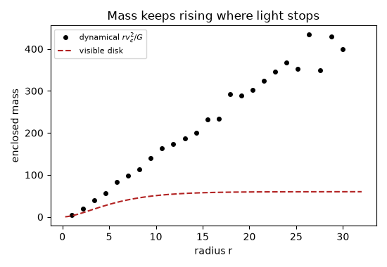
outer-curve slope d ln v / d ln r = -0.014  (Keplerian: -0.5)
r =   1.0:  M_dyn =     4.5,  M_dyn / M_visible =  1.69
r =   8.2:  M_dyn =   114.0,  M_dyn / M_visible =  2.50
r =  15.5:  M_dyn =   232.9,  M_dyn / M_visible =  4.02
r =  22.8:  M_dyn =   346.1,  M_dyn / M_visible =  5.79
r =  30.0:  M_dyn =   398.6,  M_dyn / M_visible =  6.65

Check

Beyond the optical disk the curve stays flat (slope ~0, not Keplerian -1/2), so the dynamical mass keeps growing past the visible mass.

outer_slope = np.polyfit(np.log(r_obs[outer]), np.log(v_obs[outer]), 1)[0]
assert abs(outer_slope) < 0.1
assert ratio[-1] > 5 and ratio[-1] > 3 * ratio[0]