The Navarro-Frenk-White universal halo profile

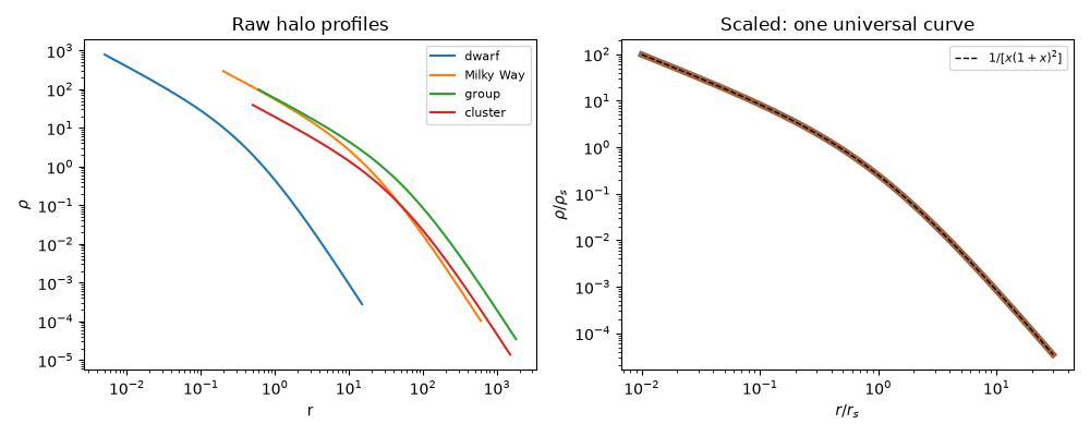
Navarro, Frenk and White (1996, 1997) found that cold-dark-matter halos in cosmological simulations share one density profile, whatever their mass,

\[\rho_{\rm NFW}(r) = \frac{\rho_s}{(r/r_s)(1+r/r_s)^2},\]

a \(r^{-1}\) cusp inside the scale radius \(r_s\) and an \(r^{-3}\) fall-off outside it. This example checks the profile’s logarithmic slope, shows that halos from dwarf to cluster scale collapse onto one curve in scaled units, and checks nfw_enclosed_mass() and nfw_potential() against direct integration of nfw_density(). Units are \(G=1\).

import matplotlib.pyplot as plt
import numpy as np

from physicskit.astro.galactic_dynamics import circular_velocity, nfw_density, nfw_enclosed_mass, nfw_potential

One shape, many halos

Four halos whose scale radii span a factor of 100 and characteristic densities a factor of 20. Raw profiles are far apart; divided by \(\rho_s\) and plotted against \(r/r_s\) they lie on top of each other.

halos = {"dwarf": (8.0, 0.5), "Milky Way": (3.0, 20.0), "group": (1.0, 60.0), "cluster": (0.4, 50.0)}

fig1, (ax1, ax2) = plt.subplots(1, 2, figsize=(10, 4))
for name, (rho_s, r_s) in halos.items():
    r = np.geomspace(0.01 * r_s, 30 * r_s, 300)
    rho = nfw_density(r, rho_s, r_s)
    ax1.loglog(r, rho, label=name)
    ax2.loglog(r / r_s, rho / rho_s, lw=4, alpha=0.5)
x = np.geomspace(0.01, 30, 300)
ax2.loglog(x, 1.0 / (x * (1 + x) ** 2), "k--", lw=1, label=r"$1/[x(1+x)^2]$")
ax1.set_xlabel("r")
ax1.set_ylabel(r"$\rho$")
ax1.set_title("Raw halo profiles")
ax1.legend(fontsize=8)
ax2.set_xlabel(r"$r/r_s$")
ax2.set_ylabel(r"$\rho/\rho_s$")
ax2.set_title("Scaled: one universal curve")
ax2.legend(fontsize=8)
fig1.tight_layout()

Cusp and fall-off: the logarithmic slope

\(d\ln\rho/d\ln r = -(1+3x)/(1+x)\), going from \(-1\) at the centre to \(-3\) far out, and passing \(-2\) exactly at \(r=r_s\).

rho_s, r_s = 1.0, 1.0
x = np.geomspace(1e-3, 1e3, 600)
slope = np.gradient(np.log(nfw_density(x, rho_s, r_s)), np.log(x))
print(f"log slope at r = 0.001 r_s: {slope[0]:.3f}")
print(f"log slope at r = r_s:       {np.interp(0.0, np.log(x), slope):.3f}")
print(f"log slope at r = 1000 r_s:  {slope[-1]:.3f}")

fig2, ax3 = plt.subplots(figsize=(5.5, 3.8))
ax3.semilogx(x, slope, color="darkorchid")
for s in (-1, -2, -3):
    ax3.axhline(s, color="0.7", lw=0.8, ls="--")
ax3.axvline(1.0, color="0.7", lw=0.8)
ax3.set_xlabel(r"$r/r_s$")
ax3.set_ylabel(r"$d\ln\rho/d\ln r$")
ax3.set_title("NFW: cusp $-1$ to fall-off $-3$")
fig2.tight_layout()

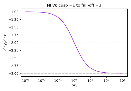
log slope at r = 0.001 r_s: -1.002
log slope at r = r_s:       -2.000
log slope at r = 1000 r_s:  -2.998

Enclosed mass, potential and circular speed

Integrating \(4\pi r^2\rho\) reproduces the closed-form \(M(<r)\); the potential’s gradient reproduces \(GM/r^2\). The circular speed peaks at \(r_{\max}\approx2.163\,r_s\).

r = np.geomspace(1e-4, 50.0, 4000)
M_numeric = np.concatenate(
    [[0.0], np.cumsum(0.5 * np.diff(r) * (4 * np.pi * r[1:] ** 2 * nfw_density(r[1:], 1, 1) + 4 * np.pi * r[:-1] ** 2 * nfw_density(r[:-1], 1, 1)))]
)
M_closed = nfw_enclosed_mass(r, rho_s, r_s)
print(f"\nmax |M_numeric - M_closed| / M_closed(r>0.1) = {np.max(np.abs(M_numeric - M_closed)[r > 0.1] / M_closed[r > 0.1]):.1e}")

g_from_phi = np.gradient(nfw_potential(r, rho_s, r_s), r)
print(f"max |dPhi/dr - GM/r^2| / (GM/r^2) (r>0.1)  = {np.max(np.abs(g_from_phi - M_closed / r**2)[r > 0.1] / (M_closed / r**2)[r > 0.1]):.1e}")

v_c = circular_velocity(r, lambda rr: nfw_enclosed_mass(rr, rho_s, r_s))
print(f"circular speed peaks at r = {r[np.argmax(v_c)]:.3f} r_s  (theory 2.163)")

plt.show()

max |M_numeric - M_closed| / M_closed(r>0.1) = 1.3e-06
max |dPhi/dr - GM/r^2| / (GM/r^2) (r>0.1)  = 2.8e-03
circular speed peaks at r = 2.163 r_s  (theory 2.163)

Check

NFW: log slope -1 (cusp), -2 at r_s, -3 far out; the closed-form mass and potential match direct integration and differentiation; v_c peaks at 2.163 r_s.

assert abs(slope[0] + 1) < 0.01 and abs(np.interp(0.0, np.log(x), slope) + 2) < 1e-3 and abs(slope[-1] + 3) < 0.01
assert np.max(np.abs(M_numeric - M_closed)[r > 0.1] / M_closed[r > 0.1]) < 1e-5
assert np.max(np.abs(g_from_phi - M_closed / r**2)[r > 0.1] / (M_closed / r**2)[r > 0.1]) < 5e-3
assert abs(r[np.argmax(v_c)] - 2.163) < 0.01