Symplectic integration and long-term N-body stability

Wisdom and Holman (1991) showed that symplectic integrators – of which the kick-drift-kick leapfrog scheme is the simplest example – keep a conservative system’s numerically computed energy oscillating within a small bound forever, rather than drifting secularly away as an ordinary (non-symplectic) integrator’s does. This is exactly what made simulations at the scale of the Millennium Simulation’s billions of particles, evolved over cosmological timescales, numerically trustworthy at all. This example integrates the same eccentric two-body orbit with NBodySystem’s symplectic leapfrog_step() for a thousand orbital periods, alongside a hand-written non-symplectic explicit-Euler stepper using the same force law (gravitational_acceleration()), and compares their energy error growth directly.

import matplotlib.pyplot as plt
import numpy as np

from physicskit.astro.nbody import NBodySystem, gravitational_acceleration
from physicskit.astro.orbital_mechanics import orbital_period, state_from_orbital_elements

An eccentric two-body orbit, run for 1000 periods

mu_total, m1, m2 = 1.0, 0.3, 0.7
a, e = 1.0, 0.5

r_vec, v_vec = state_from_orbital_elements(a, e, 0.0, 0.0, 0.0, 0.0, mu_total)
positions0 = np.array([-(m2 / mu_total) * r_vec, (m1 / mu_total) * r_vec])
velocities0 = np.array([-(m2 / mu_total) * v_vec, (m1 / mu_total) * v_vec])
masses = np.array([m1, m2])

T_period = orbital_period(a, mu_total)
steps_per_period = 200
n_periods = 1000
dt = T_period / steps_per_period
n_steps = steps_per_period * n_periods


def total_energy(positions, velocities, masses):
    kinetic = 0.5 * np.sum(masses[:, None] * velocities**2)
    r = np.linalg.norm(positions[0] - positions[1])
    potential = -masses[0] * masses[1] / r
    return kinetic + potential

The symplectic run

symplectic = NBodySystem(positions0.copy(), velocities0.copy(), masses)
E0 = symplectic.total_energy()
energy_symplectic = np.empty(n_periods + 1)
energy_symplectic[0] = E0
for p in range(n_periods):
    for _ in range(steps_per_period):
        symplectic.step(dt)
    energy_symplectic[p + 1] = symplectic.total_energy()

The non-symplectic run: hand-written explicit Euler, same force law

pos += v*dt; v += a*dt using the very same gravitational_acceleration(), so any difference in long-term behavior is due entirely to the integration scheme, not the physics.

pos_e, vel_e = positions0.copy(), velocities0.copy()
energy_euler = np.empty(n_periods + 1)
energy_euler[0] = total_energy(pos_e, vel_e, masses)
for p in range(n_periods):
    for _ in range(steps_per_period):
        acc = gravitational_acceleration(pos_e, masses)
        pos_e = pos_e + vel_e * dt
        vel_e = vel_e + acc * dt
    energy_euler[p + 1] = total_energy(pos_e, vel_e, masses)

Bounded oscillation vs. secular drift

periods = np.arange(n_periods + 1)
rel_err_symplectic = np.abs((energy_symplectic - E0) / E0)
rel_err_euler = np.abs((energy_euler - E0) / E0)

print(f"after {n_periods} periods:")
print(f"  symplectic (leapfrog) relative energy error: {rel_err_symplectic[-1]:.2e}  (max over the run: {rel_err_symplectic.max():.2e})")
print(f"  explicit Euler relative energy error:         {rel_err_euler[-1]:.2e}")

fig, ax = plt.subplots(figsize=(7, 4.5))
ax.semilogy(periods, np.maximum(rel_err_symplectic, 1e-16), color="steelblue", label="symplectic leapfrog (bounded)")
ax.semilogy(periods, np.maximum(rel_err_euler, 1e-16), color="firebrick", label="explicit Euler (secular drift)")
ax.set_xlabel("orbital periods elapsed")
ax.set_ylabel("|relative energy error|")
ax.set_title("Bounded oscillation vs. secular drift over 1000 orbits")
ax.legend()
fig.tight_layout()

plt.show()

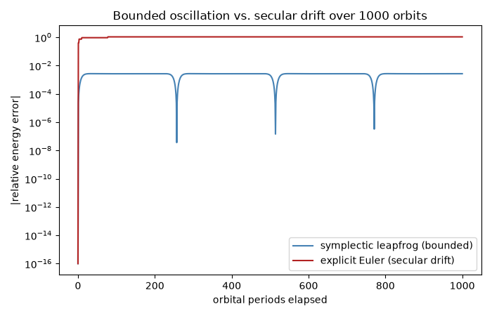
after 1000 periods:
  symplectic (leapfrog) relative energy error: 2.67e-03  (max over the run: 2.69e-03)
  explicit Euler relative energy error:         1.07e+00