Clausius’s virial theorem for a bound gravitational orbit

Clausius (1870) showed that for any bounded system interacting through conservative forces, the time-averaged kinetic energy and the time-averaged virial of the forces are related; for a system bound purely by inverse-square gravity, this reduces to

\[2\langle T\rangle + \langle U\rangle = 0,\]

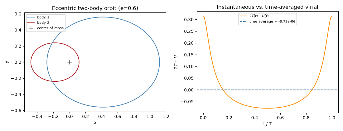
an exact statement about time averages, not an instantaneous identity (for an eccentric orbit, \(2T(t)+U(t)\) oscillates around zero without vanishing pointwise). This example builds an eccentric two-body orbit from state_from_orbital_elements(), evolves it with NBodySystem, and checks both halves of that statement directly: the instantaneous \(2T(t)+U(t)\) oscillating around zero, and its time average over one full period converging to zero far more tightly than any single instant.

import matplotlib.pyplot as plt
import numpy as np

from physicskit.astro.nbody import NBodySystem
from physicskit.astro.orbital_mechanics import orbital_period, state_from_orbital_elements

An eccentric two-body orbit, split into two masses

state_from_orbital_elements() gives the relative separation and velocity for a reduced one-body problem with \(\mu=G(m_1+m_2)\); splitting it into two individual masses about a stationary center of mass is a standard, exact construction.

mu_total, m1, m2 = 1.0, 0.3, 0.7  # m1 + m2 must equal mu_total (G=1)
a, e = 1.0, 0.6

r_vec, v_vec = state_from_orbital_elements(a, e, 0.0, 0.0, 0.0, 0.0, mu_total)
positions0 = np.array([-(m2 / mu_total) * r_vec, (m1 / mu_total) * r_vec])
velocities0 = np.array([-(m2 / mu_total) * v_vec, (m1 / mu_total) * v_vec])
masses = np.array([m1, m2])

T_period = orbital_period(a, mu_total)
dt = T_period / 4000.0
n_steps = 4000  # exactly one period

system = NBodySystem(positions0, velocities0, masses)
n = positions0.shape[0]
history = np.zeros((n_steps + 1, n, 3))
velocity_history = np.zeros((n_steps + 1, n, 3))
history[0], velocity_history[0] = system.positions, system.velocities
for k in range(n_steps):
    system.step(dt)
    history[k + 1], velocity_history[k + 1] = system.positions, system.velocities

Instantaneous vs. time-averaged \(2T+U\)

Velocity Verlet keeps position and velocity synchronized at the same time, so both can be read directly off the recorded history with no finite-difference approximation.

kinetic = 0.5 * np.sum(masses[None, :, None] * velocity_history**2, axis=(1, 2))
separations = np.linalg.norm(history[:, 0, :] - history[:, 1, :], axis=1)
potential = -masses[0] * masses[1] / separations
virial_quantity = 2.0 * kinetic + potential

t = np.arange(n_steps + 1) * dt
time_avg = np.trapezoid(virial_quantity, t) / (t[-1] - t[0])
print(f"orbital period: T = {T_period:.6f}")
print(f"instantaneous 2T+U: min={virial_quantity.min():.4f}, max={virial_quantity.max():.4f} (oscillates around zero, not pointwise zero)")
print(f"time-averaged 2T+U over one full period: {time_avg:.6f}  (this is what Clausius's theorem actually predicts is zero)")

fig, (ax1, ax2) = plt.subplots(1, 2, figsize=(11, 4.2))
ax1.plot(history[:, 0, 0], history[:, 0, 1], color="steelblue", label="body 1")
ax1.plot(history[:, 1, 0], history[:, 1, 1], color="firebrick", label="body 2")
ax1.plot(0, 0, "k+", ms=10, label="center of mass")
ax1.set_xlabel("x")
ax1.set_ylabel("y")
ax1.set_title(f"Eccentric two-body orbit (e={e})")
ax1.set_aspect("equal")
ax1.legend(fontsize=8)

ax2.plot(t / T_period, virial_quantity, color="darkorange", label=r"$2T(t)+U(t)$")
ax2.axhline(0.0, color="0.4", lw=1)
ax2.axhline(time_avg, color="steelblue", ls="--", label=f"time average = {time_avg:.2e}")
ax2.set_xlabel("t / T")
ax2.set_ylabel(r"$2T+U$")
ax2.set_title("Instantaneous vs. time-averaged virial")
ax2.legend(fontsize=8)
fig.tight_layout()

plt.show()

orbital period: T = 6.283185
instantaneous 2T+U: min=-0.0787, max=0.3150 (oscillates around zero, not pointwise zero)
time-averaged 2T+U over one full period: -0.000009  (this is what Clausius's theorem actually predicts is zero)