Kepler’s laws of planetary motion

Kepler’s three laws were extracted purely from observation – Tycho Brahe’s measurements of Mars for the first two (Astronomia Nova, 1609), and the periods and distances of the six known planets for the third (Harmonices Mundi, 1619):

1. each planet moves on an ellipse with the Sun at one focus;

2. the Sun-planet line sweeps out equal areas in equal times;

3. \(T^2 \propto a^3\).

This example illustrates each law in turn, using nothing but orbital geometry: state_from_orbital_elements() for the ellipse, Kepler’s own equation \(M = E - e\sin E\) for the timing, and orbital_period() against the planetary data Kepler worked from.

import matplotlib.pyplot as plt
import numpy as np

from physicskit.astro.orbital_mechanics import orbital_period, state_from_orbital_elements

First law: an ellipse with the Sun at one focus

Gravitational units, \(\mu=GM=1\). An eccentricity of 0.6 (far larger than Mars’s 0.093) makes the offset of the Sun from the centre visually obvious.

mu = 1.0
a, e = 1.5, 0.6
b = a * np.sqrt(1.0 - e**2)

nu = np.linspace(0.0, 2.0 * np.pi, 400)
r_vec = np.array([state_from_orbital_elements(a, e, 0.0, 0.0, 0.0, v, mu)[0] for v in nu])

fig1, ax1 = plt.subplots(figsize=(5.5, 5.5))
ax1.plot(r_vec[:, 0], r_vec[:, 1], color="steelblue", lw=2)
ax1.plot(0, 0, "o", color="orange", ms=14, label="Sun (occupied focus)")
ax1.plot(-2 * a * e, 0, "x", color="gray", ms=9, label="empty focus")
ax1.plot(-a * e, 0, "+", color="black", ms=9, label="centre")
ax1.set_xlabel("x")
ax1.set_ylabel("y")
ax1.set_title(f"Kepler's first law: ellipse, a={a}, e={e}")
ax1.set_aspect("equal")
ax1.legend(loc="upper right", fontsize=8)
fig1.tight_layout()

# The defining property of an ellipse: the distances to the two foci sum
# to 2a at every point.
focal_sum = np.linalg.norm(r_vec[:, :2], axis=1) + np.linalg.norm(r_vec[:, :2] - [-2 * a * e, 0.0], axis=1)
print(f"r_Sun + r_empty over the orbit: min {focal_sum.min():.6f}, max {focal_sum.max():.6f}, 2a = {2 * a}")

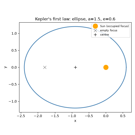
r_Sun + r_empty over the orbit: min 3.000000, max 3.000000, 2a = 3.0

Second law: equal areas in equal times

Kepler timed the orbit with his own equation: the mean anomaly \(M = 2\pi t/T\) grows uniformly in time, and the eccentric anomaly \(E\) solves \(M = E - e\sin E\) (here by Newton iteration). Twelve equal time steps then give twelve sectors that are long and thin near periapsis and short and wide near apoapsis – but all of the same area, \(\pi ab/12\).

n_sectors = 12
M = np.linspace(0.0, 2.0 * np.pi, n_sectors + 1)
E = M.copy()
for _ in range(50):
    E -= (E - e * np.sin(E) - M) / (1.0 - e * np.cos(E))
nu_k = 2.0 * np.arctan2(np.sqrt(1.0 + e) * np.sin(E / 2), np.sqrt(1.0 - e) * np.cos(E / 2))

fig2, ax2 = plt.subplots(figsize=(5.5, 5.5))
colors = plt.cm.viridis(np.linspace(0.1, 0.9, n_sectors))
areas = []
for k in range(n_sectors):
    nu_lo, nu_hi = nu_k[k], nu_k[k + 1]
    if nu_hi <= nu_lo:
        nu_hi += 2.0 * np.pi
    arc = np.array([state_from_orbital_elements(a, e, 0.0, 0.0, 0.0, v, mu)[0][:2] for v in np.linspace(nu_lo, nu_hi, 200)])
    sector = np.vstack([[0.0, 0.0], arc])
    ax2.fill(sector[:, 0], sector[:, 1], color=colors[k], alpha=0.8, lw=0.5, edgecolor="white")
    # Shoelace formula for the sector's area.
    x, y = sector[:, 0], sector[:, 1]
    areas.append(0.5 * abs(np.dot(x, np.roll(y, -1)) - np.dot(y, np.roll(x, -1))))
ax2.plot(0, 0, "o", color="orange", ms=12)
ax2.set_title("Kepler's second law: 12 equal-time sectors")
ax2.set_aspect("equal")
ax2.set_xlabel("x")
ax2.set_ylabel("y")
fig2.tight_layout()

print(f"\nsector areas: {np.round(areas, 5).tolist()}")
print(f"expected pi*a*b/{n_sectors} = {np.pi * a * b / n_sectors:.5f}")

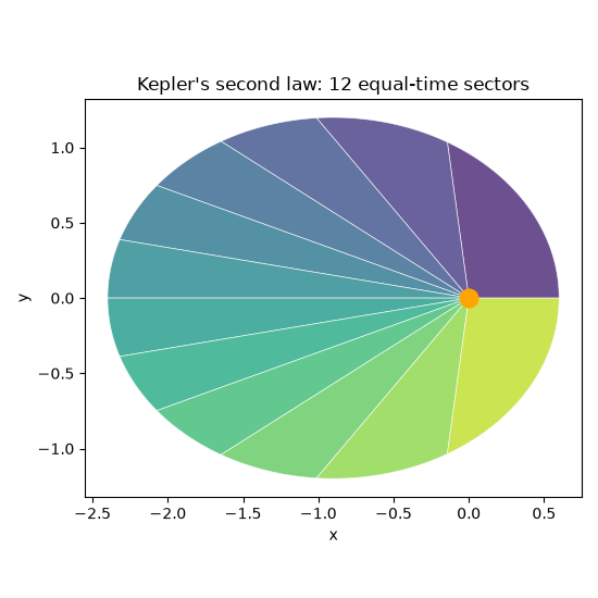
sector areas: [0.47123, 0.47124, 0.47124, 0.47124, 0.47124, 0.47124, 0.47124, 0.47124, 0.47124, 0.47124, 0.47124, 0.47123]
expected pi*a*b/12 = 0.47124

Third law: \(T^2 \propto a^3\) for the planets Kepler knew

In units of AU and years, \(\mu_\odot = 4\pi^2\), and orbital_period() reproduces the observed periods of all six naked-eye planets – the same regularity Kepler found in the tables of his day.

planets = ["Mercury", "Venus", "Earth", "Mars", "Jupiter", "Saturn"]
a_obs = np.array([0.387, 0.723, 1.000, 1.524, 5.203, 9.537])  # AU
T_obs = np.array([0.241, 0.615, 1.000, 1.881, 11.862, 29.457])  # yr
mu_sun = 4.0 * np.pi**2
T_law = np.array([orbital_period(av, mu_sun) for av in a_obs])

print(f"\n{'planet':<8} {'a [AU]':>7} {'T obs [yr]':>11} {'T law [yr]':>11} {'T^2/a^3':>8}")
for name, av, To, Tl in zip(planets, a_obs, T_obs, T_law):
    print(f"{name:<8} {av:7.3f} {To:11.3f} {Tl:11.3f} {To**2 / av**3:8.4f}")

a_grid = np.geomspace(0.3, 12.0, 100)
fig3, ax3 = plt.subplots(figsize=(5.5, 4.5))
ax3.loglog(a_grid, [orbital_period(av, mu_sun) for av in a_grid], "--", color="orange", label=r"$T = 2\pi\sqrt{a^3/\mu_\odot}$")
ax3.loglog(a_obs, T_obs, "o", color="steelblue", label="observed")
for name, av, To in zip(planets, a_obs, T_obs):
    ax3.annotate(name, (av, To), textcoords="offset points", xytext=(6, -10), fontsize=8)
ax3.set_xlabel("semi-major axis $a$ [AU]")
ax3.set_ylabel("period $T$ [yr]")
ax3.set_title("Kepler's third law (slope 3/2)")
ax3.legend(loc="upper left")
fig3.tight_layout()

plt.show()

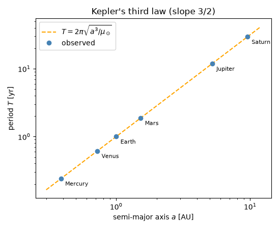
planet    a [AU]  T obs [yr]  T law [yr]  T^2/a^3
Mercury    0.387       0.241       0.241   1.0021
Venus      0.723       0.615       0.615   1.0008
Earth      1.000       1.000       1.000   1.0000
Mars       1.524       1.881       1.881   0.9996
Jupiter    5.203      11.862      11.868   0.9990
Saturn     9.537      29.457      29.452   1.0003

Check

First law: r + r’ = 2a. Second law: equal areas pi a b / 12 in equal times. Third law: T^2 / a^3 = 1 yr^2 / AU^3 for the planets.

np.testing.assert_allclose(focal_sum, 2 * a, rtol=1e-9)
np.testing.assert_allclose(areas, np.pi * a * b / n_sectors, rtol=2e-3)
np.testing.assert_allclose(T_obs**2 / a_obs**3, 1, rtol=3e-3)