Newton’s law of universal gravitation

Newton’s Principia (1687) replaced Kepler’s three empirical rules with a single dynamical law: every pair of masses attracts along the line joining them with

\[\vec F = -\frac{G m_1 m_2}{r^2}\,\hat r.\]

This example starts from that force alone. It checks the inverse-square scaling and the equal-and-opposite pairing directly with gravitational_acceleration(), then integrates a two-body system from arbitrary initial conditions with NBodySystem – never imposing an orbit shape – and shows that Kepler’s laws come out as consequences: a closed conic with constant elements, conserved angular momentum (equal areas), and a period fixed by \(\mu = G(M+m)\).

import matplotlib.pyplot as plt
import numpy as np

from physicskit.astro.nbody import NBodySystem, gravitational_acceleration
from physicskit.astro.orbital_mechanics import orbital_elements_from_state, orbital_period, vis_viva_speed

The force law: inverse square, equal and opposite

Place a test mass at distances spanning two decades from a unit mass. On a log-log plot the acceleration is a straight line of slope \(-2\). The pair of accelerations also satisfies Newton’s third law, \(m_1\vec a_1 = -m_2\vec a_2\), for any mass ratio.

G = 1.0
distances = np.geomspace(0.1, 10.0, 25)
acc = np.array([np.linalg.norm(gravitational_acceleration(np.array([[0.0, 0, 0], [d, 0, 0]]), np.array([1.0, 1e-6]), G=G)[1]) for d in distances])
slope = np.polyfit(np.log(distances), np.log(acc), 1)[0]
print(f"fitted power law |a| ~ r^{slope:.6f}  (Newton: r^-2)")

masses_pair = np.array([3.0, 0.5])
acc_pair = gravitational_acceleration(np.array([[0.0, 0, 0], [1.2, 0.7, -0.3]]), masses_pair, G=G)
print(f"m1*a1 + m2*a2 = {masses_pair[0] * acc_pair[0] + masses_pair[1] * acc_pair[1]}  (third law: zero)")

fig1, ax1 = plt.subplots(figsize=(5, 4.2))
ax1.loglog(distances, acc, "o", color="steelblue", label="gravitational_acceleration")
ax1.loglog(distances, G / distances**2, "--", color="orange", label=r"$GM/r^2$")
ax1.set_xlabel("separation $r$")
ax1.set_ylabel("acceleration $|a|$")
ax1.set_title("Inverse-square law")
ax1.legend()
fig1.tight_layout()

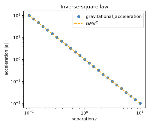
fitted power law |a| ~ r^-2.000000  (Newton: r^-2)
m1*a1 + m2*a2 = [ 0.00000000e+00 -5.55111512e-17  0.00000000e+00]  (third law: zero)

Integrating the force: the orbit emerges

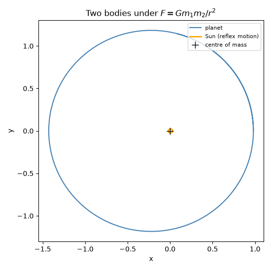
A heavy “Sun” and a light “planet” (mass ratio 50:1, so the Sun’s own reflex motion is visible) start from an arbitrary position and velocity. Only the force law is integrated. The relative orbit nevertheless closes on itself as an ellipse with the Sun at a focus, and the two bodies circle their common centre of mass.

M, m = 1.0, 0.02
mu = G * (M + m)
positions = np.array([[0.0, 0.0, 0.0], [1.0, 0.0, 0.0]])
velocities = np.array([[0.0, 0.0, 0.0], [0.0, 1.1, 0.0]])
# Move to the centre-of-mass frame so the system doesn't drift.
masses = np.array([M, m])
velocities -= (masses[:, None] * velocities).sum(axis=0) / masses.sum()
positions -= (masses[:, None] * positions).sum(axis=0) / masses.sum()

system = NBodySystem(positions, velocities, masses, G=G)
E0, L0 = system.total_energy(), system.total_angular_momentum()

dt, n_steps = 1e-3, 10000
rel_r, rel_v = [], []
history = np.zeros((n_steps + 1, 2, 3))
history[0] = system.positions
for k in range(n_steps):
    rel_r.append(system.positions[1] - system.positions[0])
    rel_v.append(system.velocities[1] - system.velocities[0])
    system.step(dt)
    history[k + 1] = system.positions
rel_r, rel_v = np.array(rel_r), np.array(rel_v)

fig2, ax2 = plt.subplots(figsize=(5.5, 5.5))
ax2.plot(history[:, 1, 0], history[:, 1, 1], color="steelblue", lw=1.5, label="planet")
ax2.plot(history[:, 0, 0], history[:, 0, 1], color="orange", lw=2, label="Sun (reflex motion)")
ax2.plot(0, 0, "+", color="black", ms=10, label="centre of mass")
ax2.set_aspect("equal")
ax2.set_xlabel("x")
ax2.set_ylabel("y")
ax2.set_title("Two bodies under $F = Gm_1m_2/r^2$")
ax2.legend(loc="upper right", fontsize=8)
fig2.tight_layout()

Kepler’s laws as consequences

• First law. The orbital elements recovered from the relative state at every step are constant: the trajectory is one fixed ellipse.

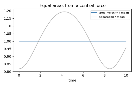
• Second law. The areal velocity \(|\vec r\times\vec v|/2\) is constant – angular momentum conservation for a central force.

• Third law. The measured period matches \(2\pi\sqrt{a^3/G(M+m)}\), the constant Kepler could only fit.

elements = np.array([orbital_elements_from_state(r, v, mu)[:2] for r, v in zip(rel_r, rel_v)])
a_fit, e_fit = elements[:, 0].mean(), elements[:, 1].mean()
print(f"\na: mean {a_fit:.6f}, spread {np.ptp(elements[:, 0]):.2e}")
print(f"e: mean {e_fit:.6f}, spread {np.ptp(elements[:, 1]):.2e}")

areal = 0.5 * np.linalg.norm(np.cross(rel_r, rel_v), axis=1)
print(f"areal velocity: mean {areal.mean():.6f}, relative spread {np.ptp(areal) / areal.mean():.2e}")

# Period: time for the separation vector to sweep a full 2*pi.
angle = np.unwrap(np.arctan2(rel_r[:, 1], rel_r[:, 0]))
T_measured = np.interp(2.0 * np.pi, angle, np.arange(len(angle)) * dt)
print(f"period: measured {T_measured:.5f}, Newton 2*pi*sqrt(a^3/G(M+m)) = {orbital_period(a_fit, mu):.5f}")

r_mag = np.linalg.norm(rel_r, axis=1)
v_mag = np.linalg.norm(rel_v, axis=1)
print(f"vis-viva speed error along orbit: max {np.max(np.abs(v_mag - [vis_viva_speed(r, a_fit, mu) for r in r_mag])):.2e}")
print(f"energy drift {abs(system.total_energy() - E0):.2e}, angular-momentum drift {np.linalg.norm(system.total_angular_momentum() - L0):.2e}")

fig3, ax3 = plt.subplots(figsize=(5.5, 3.5))
t = np.arange(len(areal)) * dt
ax3.plot(t, areal / areal.mean(), color="steelblue", label="areal velocity / mean")
ax3.plot(t, r_mag / r_mag.mean(), color="gray", alpha=0.6, label="separation / mean")
ax3.set_xlabel("time")
ax3.set_title("Equal areas from a central force")
ax3.legend(fontsize=8)
fig3.tight_layout()

plt.show()

a: mean 1.228916, spread 1.58e-07
e: mean 0.186275, spread 3.34e-07
areal velocity: mean 0.550000, relative spread 1.17e-14
period: measured 8.47546, Newton 2*pi*sqrt(a^3/G(M+m)) = 8.47545
vis-viva speed error along orbit: max 3.20e-08
energy drift 7.62e-10, angular-momentum drift 7.63e-17

Check

Inverse-square force, action = reaction, and the conserved Kepler elements, areal velocity and period of the resulting two-body orbit.

assert abs(slope + 2) < 1e-9
assert np.allclose(masses_pair[0] * acc_pair[0] + masses_pair[1] * acc_pair[1], 0, atol=1e-12)
assert np.ptp(elements[:, 0]) < 1e-5 and np.ptp(elements[:, 1]) < 1e-5
assert np.ptp(areal) / areal.mean() < 1e-10
assert abs(T_measured / orbital_period(a_fit, mu) - 1) < 1e-4