Saving and Loading Results

Long simulations (a fine basin-of-attraction grid, a long Lyapunov-spectrum integration, a large parameter sweep) are worth keeping around instead of recomputing. physicskit.chaos.utils.io provides two small, generic building blocks for this: save_system_config() / load_system_config() round-trip a system’s class and constructor parameters through JSON (using the same __init__ introspection that already powers every system’s repr()), and save_arrays() / load_arrays() save any named arrays (a trajectory, a basin grid, a Poincare section) to a plain .npz archive. The system used to demonstrate this is the Lorenz attractor,

\[\dot{x} = \sigma (y - x), \qquad \dot{y} = x (\rho - z) - y, \qquad \dot{z} = x y - \beta z,\]

with the classic parameters \(\sigma=10\), \(\rho=28\), \(\beta=8/3\) – but the save/load round-trip below works identically for any DynamicalSystem.

from __future__ import annotations

import tempfile
from pathlib import Path

import matplotlib.pyplot as plt

from physicskit.chaos.systems.continuous import Lorenz
from physicskit.chaos.utils.io import load_arrays, load_system_config, save_arrays, save_system_config

Saving a system’s configuration

Only the class and its constructor parameters are saved – not the trajectory itself – so the file is tiny and the system can be re-integrated identically (or with different n_steps/dt) later.

tmp_dir = Path(tempfile.mkdtemp())
system = Lorenz(sigma=10.0, rho=28.0, beta=8.0 / 3.0)
config_path = tmp_dir / "lorenz_config.json"
save_system_config(system, config_path)
print(config_path.read_text())

restored = load_system_config(config_path)
print(f"restored: {restored!r}")
assert restored.sigma == system.sigma and restored.rho == system.rho

{
  "module": "physicskit.chaos.systems.continuous",
  "class": "Lorenz",
  "params": {
    "sigma": 10.0,
    "rho": 28.0,
    "beta": 2.6666666666666665
  }
}
restored: Lorenz(sigma=10.0, rho=28.0, beta=2.6666666666666665)

Saving trajectory data

save_arrays accepts any set of named arrays and stores them together in one .npz file; load_arrays hands them back as a plain dict.

t, states = restored.trajectory(n_steps=5000, dt=0.01)
data_path = tmp_dir / "lorenz_run.npz"
save_arrays(data_path, t=t, states=states)

loaded = load_arrays(data_path)
print(f"loaded arrays: {list(loaded.keys())}, states shape = {loaded['states'].shape}")

fig, ax = plt.subplots(figsize=(6, 5))
ax.plot(loaded["states"][:, 0], loaded["states"][:, 2], lw=0.4)
ax.set_xlabel("x")
ax.set_ylabel("z")
ax.set_title("Trajectory reloaded from disk, unchanged")

plt.show()

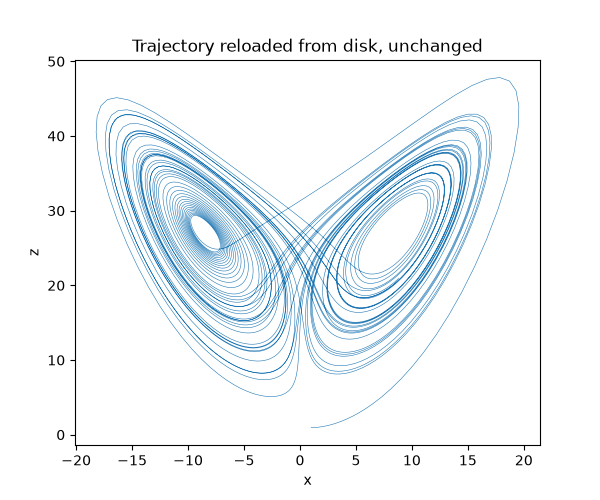
loaded arrays: ['t', 'states'], states shape = (5001, 3)