Symplectic vs. Non-Symplectic Integrators: Long-Horizon Energy Drift

For conservative (Hamiltonian) systems, the choice of integrator matters far more over long integration horizons than local per-step accuracy suggests. 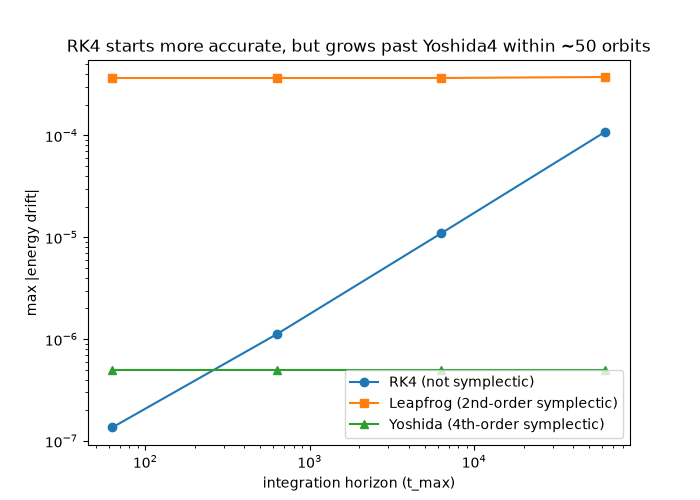This example integrates a simple, exactly-solvable Kepler orbit with three integrators from physicskit.chaos.core.integrators – RK4, the 2nd-order symplectic leapfrog, and the 4th-order symplectic Yoshida scheme – and compares how their energy-conservation error behaves as the integration horizon grows. RK4’s error grows secularly (roughly proportional to integration time), while the symplectic integrators’ error stays bounded regardless of how long you integrate, because they exactly preserve phase-space volume at every step: over a handful of orbits RK4 actually has the smallest error of the three, but by a few dozen orbits it has already grown past Yoshida4’s, and keeps growing indefinitely from there. A second figure makes the abstract “energy drift” number concrete: since a Kepler orbit’s specific energy fixes its semi-major axis, tracking the aphelion distance orbit by orbit shows RK4’s secular energy error directly shrinking the orbit over time, while Yoshida4’s bounded error keeps it flat.

import matplotlib.pyplot as plt
import numpy as np
from numba import njit

from physicskit.chaos.core.integrators import leapfrog_integrate, rk4_integrate, yoshida4_integrate

A Kepler orbit

A planet of negligible mass orbiting a unit point mass under Newtonian gravity, in units where G*M = 1, so the position \(\mathbf{r}=(x,y)\) obeys

\[\ddot{\mathbf{r}} = -\frac{\mathbf{r}}{|\mathbf{r}|^3},\]

with conserved specific orbital energy \(E = \tfrac{1}{2}|\dot{ \mathbf{r}}|^2 - 1/|\mathbf{r}|\). Gravity here depends only on position, so this is a separable Hamiltonian – exactly the kind of system the symplectic integrators are built for.

@njit(cache=True)
def _kepler_force(pos, t, params):
    r = np.sqrt(pos[0] ** 2 + pos[1] ** 2)
    return -pos / r**3


@njit(cache=True)
def _kepler_rhs(state, t, params):
    x, y, vx, vy = state[0], state[1], state[2], state[3]
    r = np.sqrt(x * x + y * y)
    out = np.empty(4)
    out[0], out[1] = vx, vy
    out[2], out[3] = -x / r**3, -y / r**3
    return out


def _kepler_energy(pos, vel):
    r = np.hypot(pos[:, 0], pos[:, 1])
    v2 = vel[:, 0] ** 2 + vel[:, 1] ** 2
    return 0.5 * v2 - 1.0 / r


# An eccentric orbit (e = 0.6, semi-major axis a = 1, period 2*pi), starting
# at perihelion (r_min = a*(1-e) = 0.4) with the vis-viva speed
# v_peri = sqrt(2/r_min - 1/a) = 2.0.
pos0 = np.array([0.4, 0.0])
vel0 = np.array([0.0, 2.0])
params = np.array([0.0])
dt = 0.01

Integrate over successively longer horizons

The orbital period here is 2*pi ~= 6.283; these horizons span roughly 10 to 10,000 orbits.

period = 2.0 * np.pi
horizons = [int(n_orbits * period / dt) for n_orbits in (10, 100, 1000, 10000)]
drift_rk4, drift_lf, drift_y4 = [], [], []

for n_steps in horizons:
    _, states = rk4_integrate(_kepler_rhs, np.concatenate([pos0, vel0]), 0.0, dt, n_steps, params)
    e_rk4 = 0.5 * (states[:, 2] ** 2 + states[:, 3] ** 2) - 1.0 / np.hypot(states[:, 0], states[:, 1])
    drift_rk4.append(np.max(np.abs(e_rk4 - e_rk4[0])))

    _, pos_lf, vel_lf = leapfrog_integrate(_kepler_force, pos0, vel0, 0.0, dt, n_steps, params)
    e_lf = _kepler_energy(pos_lf, vel_lf)
    drift_lf.append(np.max(np.abs(e_lf - e_lf[0])))

    _, pos_y4, vel_y4 = yoshida4_integrate(_kepler_force, pos0, vel0, 0.0, dt, n_steps, params)
    e_y4 = _kepler_energy(pos_y4, vel_y4)
    drift_y4.append(np.max(np.abs(e_y4 - e_y4[0])))

Plot

t_max = np.array(horizons) * dt
fig, ax = plt.subplots(figsize=(7, 5))
ax.loglog(t_max, drift_rk4, "o-", label="RK4 (not symplectic)")
ax.loglog(t_max, drift_lf, "s-", label="Leapfrog (2nd-order symplectic)")
ax.loglog(t_max, drift_y4, "^-", label="Yoshida (4th-order symplectic)")
ax.set_xlabel("integration horizon (t_max)")
ax.set_ylabel("max |energy drift|")
ax.set_title("RK4 starts more accurate, but grows past Yoshida4 within ~50 orbits")
ax.legend()

<matplotlib.legend.Legend object at 0x136c4d280>

What the drift actually does to the orbit: a shrinking aphelion

The log-log plot above only shows a scalar (the worst energy error) at a handful of horizons; it doesn’t show what that error actually does to the orbit. A negative specific energy fixes the semi-major axis via \(E=-1/(2a)\), so any energy drift directly rescales the orbit’s size; tracking the aphelion distance (the local maxima of \(r(t)\), one per orbit) makes that rescaling visible one orbit at a time. Over 1000 orbits at the same dt used above, RK4’s aphelion visibly creeps inward as its secular energy error accumulates, while Yoshida4’s stays flat – bounded noise at the \(10^{-6}\) level, with no trend at all.

n_orbits_shape = 1000
n_steps_shape = int(n_orbits_shape * period / dt)

_, states_rk4_shape = rk4_integrate(_kepler_rhs, np.concatenate([pos0, vel0]), 0.0, dt, n_steps_shape, params)
_, pos_y4_shape, vel_y4_shape = yoshida4_integrate(_kepler_force, pos0, vel0, 0.0, dt, n_steps_shape, params)


def _aphelion_per_orbit(pos):
    """Distance from the origin at each local maximum of r(t) (one per orbit)."""
    r = np.hypot(pos[:, 0], pos[:, 1])
    is_max = (r[1:-1] > r[:-2]) & (r[1:-1] > r[2:])
    return r[1:-1][is_max]


aphelion_rk4 = _aphelion_per_orbit(states_rk4_shape[:, :2])
aphelion_y4 = _aphelion_per_orbit(pos_y4_shape)
print(
    f"Aphelion distance (true value = 1.6): RK4 drifts from {aphelion_rk4[0]:.6f} to "
    f"{aphelion_rk4[-1]:.6f}; Yoshida4 stays within {np.ptp(aphelion_y4):.1e} of {aphelion_y4[0]:.6f}"
)

fig2, ax2 = plt.subplots(figsize=(8, 5))
ax2.plot(np.arange(1, len(aphelion_rk4) + 1), aphelion_rk4, color="crimson", label="RK4 (not symplectic)")
ax2.plot(np.arange(1, len(aphelion_y4) + 1), aphelion_y4, color="steelblue", label="Yoshida4 (4th-order symplectic)")
ax2.axhline(1.6, color="gray", lw=0.8, ls="--", label="exact aphelion = 1.6")
ax2.set_xlabel("orbit number")
ax2.set_ylabel("aphelion distance")
ax2.set_title(f"Same Kepler orbit, same dt: RK4's aphelion creeps inward over {n_orbits_shape} orbits")
ax2.legend()
fig2.tight_layout()

plt.show()

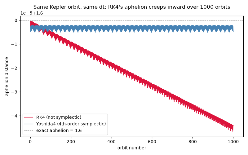
Aphelion distance (true value = 1.6): RK4 drifts from 1.600000 to 1.599956; Yoshida4 stays within 2.9e-06 of 1.599998