Ellipse Billiard (Integrable, with Caustics)

A billiard particle moves in a straight line at constant speed inside a closed boundary and undergoes specular reflection, \(\mathbf{v}' = \mathbf{v} - 2(\mathbf{v}\cdot\mathbf{n})\,\mathbf{n}\), whenever it strikes the boundary. Here the boundary is the ellipse

\[\frac{x^2}{a^2} + \frac{y^2}{b^2} = 1,\]

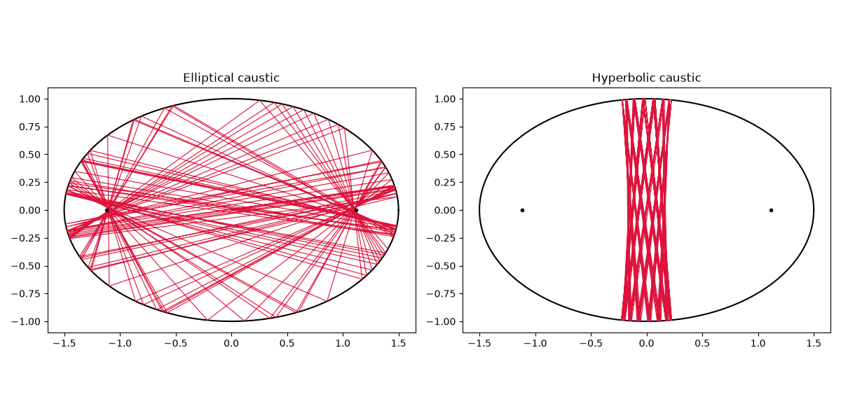
with semi-major axis \(a\) and semi-minor axis \(b\), and foci at \((\pm c, 0)\), \(c = \sqrt{a^2 - b^2}\). The elliptical billiard is integrable, like the Circle and Rectangle, but illustrates a richer piece of the theory: every trajectory stays tangent to a single confocal caustic for all time – either a confocal ellipse (for trajectories that never pass between the two foci) or a confocal hyperbola (for trajectories that do). This example plots a trajectory of each kind and the resulting Poincare section.

import matplotlib.pyplot as plt

from physicskit.chaos.systems.billiards import EllipseBilliard
from physicskit.chaos.visualizers.dynamic_plots import animate_billiard_trajectory
from physicskit.chaos.visualizers.phase_space import plot_billiard_trajectory, plot_poincare_section

billiard = EllipseBilliard(semi_major=1.5, semi_minor=1.0)
f1, f2 = billiard.foci()

Animation

Watch the ray trace out its confocal elliptical caustic – the envelope of lines it stays perpetually tangent to – one bounce at a time.

anim = animate_billiard_trajectory(billiard, pos=(0.0, 0.0), vel=(1.0, 0.15), n_bounces=100, interval=50)

plt.show()

To save the animation to a file instead of (or in addition to) displaying it interactively, use e.g.:

anim.save("ellipse_billiard_animation.gif", writer="pillow", fps=20)

Two families of caustics

A trajectory that never crosses the segment joining the foci stays tangent to a confocal ellipse (left); one that does cross it stays tangent to a confocal hyperbola (right).

fig, axes = plt.subplots(1, 2, figsize=(12, 6))

plot_billiard_trajectory(billiard, pos=(0.0, 0.0), vel=(1.0, 0.15), n_bounces=100, ax=axes[0])
axes[0].plot(*f1, "k.", *f2, "k.")
axes[0].set_title("Elliptical caustic")

plot_billiard_trajectory(billiard, pos=(0.0, 0.0), vel=(0.15, 1.0), n_bounces=100, ax=axes[1])
axes[1].plot(*f1, "k.", *f2, "k.")
axes[1].set_title("Hyperbolic caustic")
fig.tight_layout()

Poincare section

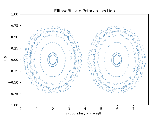
Every ray traces out a smooth invariant curve, just as for the Circle and Rectangle billiards – the signature of integrability. Rays confined to elliptical caustics produce closed curves; rays confined to hyperbolic caustics produce the “wavy” curves crossing the sin(phi) = 0 axis.

fig2, ax2 = plot_poincare_section(billiard, n_rays=15, n_bounces=200)

plt.show()