Comparing All Five Billiards

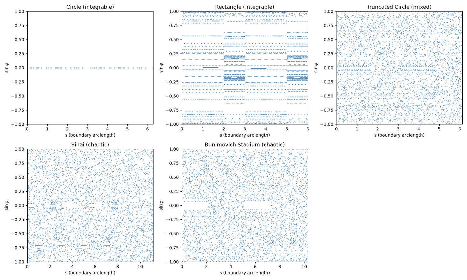
Every billiard here is a point particle moving in a straight line at constant speed inside a closed boundary, undergoing specular reflection

\[\mathbf{v}' = \mathbf{v} - 2(\mathbf{v}\cdot\mathbf{n})\,\mathbf{n}\]

whenever it strikes the boundary; the five shapes below differ only in that boundary’s geometry: a disk \(x^2+y^2=r^2\) (Circle), a rectangle \(|x|\le w/2,\ |y|\le h/2\) (Rectangle), a disk with a flat chord cut off (Truncated Circle), a square cell with a circular scatterer removed from its center (Sinai), and two semicircular caps joined by straight edges (Bunimovich Stadium). This is a side-by-side comparison of the Poincare section for every billiard shape physicskit.chaos ships, from fully integrable (Circle, Rectangle) through mixed (Truncated Circle) to fully chaotic (Sinai, Bunimovich Stadium).

import matplotlib.pyplot as plt

from physicskit.chaos.systems.billiards import (
    BunimovichStadium,
    CircleBilliard,
    RectangleBilliard,
    SinaiBilliard,
    TruncatedCircleBilliard,
)
from physicskit.chaos.visualizers.phase_space import plot_poincare_section

Build one instance of each billiard and plot its Poincare section into its own subplot, using the ax= parameter of physicskit.chaos.visualizers.phase_space.plot_poincare_section() to draw into a shared figure.

billiards = {
    "Circle (integrable)": CircleBilliard(radius=1.0),
    "Rectangle (integrable)": RectangleBilliard(width=2.0, height=1.0),
    "Truncated Circle (mixed)": TruncatedCircleBilliard(radius=1.0, cut=0.3),
    "Sinai (chaotic)": SinaiBilliard(cell_size=2.0, scatterer_radius=0.5),
    "Bunimovich Stadium (chaotic)": BunimovichStadium(radius=1.0, straight_length=2.0),
}

fig, axes = plt.subplots(2, 3, figsize=(15, 9))
for ax, (name, billiard) in zip(axes.flat, billiards.items()):
    plot_poincare_section(billiard, n_rays=25, n_bounces=150, ax=ax, s=1.0)
    ax.set_title(name)
axes.flat[-1].axis("off")
fig.tight_layout()

plt.show()