Analyzing a Raw Time Series (No Equations Required)

Every other chaos-diagnostic tool in this gallery works on a DynamicalSystem with known equations of motion. Real experimental data doesn’t come with equations attached – this example instead analyzes a single scalar time series, \(x(t)\), treating its true source – here the Lorenz system, \(\dot{x}=\sigma(y-x)\), \(\dot{y}=x(\rho-z)-y\), \(\dot{z}=xy-\beta z\) – as unknown, and using only \(x(t)\) itself. It reconstructs an equivalent phase-space attractor by delay-coordinate (Takens) embedding,

\[\mathbf{y}(t) = \left(x(t),\ x(t+\tau),\ \ldots,\ x(t+(d-1)\tau)\right),\]

then estimates the largest Lyapunov exponent from the reconstruction with the Rosenstein algorithm, tests whether the series shows genuine nonlinear structure with IAAFT surrogate-data significance testing, and examines its spectral diagnostics (power spectrum and autocorrelation).

import matplotlib.pyplot as plt
import numpy as np

from physicskit.chaos.systems.continuous import Lorenz
from physicskit.chaos.utils.spectral import autocorrelation, power_spectrum
from physicskit.chaos.utils.timeseries import (
    average_log_divergence,
    delay_embed,
    rosenstein_lyapunov,
    surrogate_test,
)

The “observed” data

Only the scalar x(t) is used from here on – the y and z coordinates, and the equations of motion themselves, are treated as unknown.

system = Lorenz()
dt = 0.01
_, states = system.trajectory(n_steps=20000, dt=dt)
x = states[1000:, 0]

fig, ax = plt.subplots(figsize=(9, 3.5))
ax.plot(np.arange(x.size) * dt, x, lw=0.5)
ax.set_xlabel("t")
ax.set_ylabel("x(t)")
ax.set_title("The only data available: a single scalar time series")

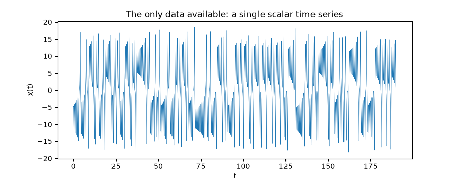
Text(0.5, 1.0, 'The only data available: a single scalar time series')

Reconstructing the attractor: delay embedding

Takens’ theorem guarantees that, for a generic choice of embedding dimension and delay, a delay-coordinate embedding of a single observed variable reconstructs an attractor equivalent to the original – no other variables or equations needed.

embedded = delay_embed(x, dim=3, tau=10)

fig2 = plt.figure(figsize=(6, 6))
ax2 = fig2.add_subplot(projection="3d")
ax2.plot(embedded[:, 0], embedded[:, 1], embedded[:, 2], lw=0.2, color="darkorange")
ax2.set_xlabel("x(t)")
ax2.set_ylabel("x(t + tau)")
ax2.set_zlabel("x(t + 2*tau)")
ax2.set_title("Delay-embedded reconstruction (recognizably the Lorenz attractor)")

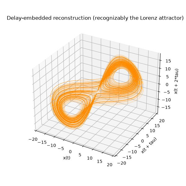
Text(0.5, 1.0, 'Delay-embedded reconstruction (recognizably the Lorenz attractor)')

The largest Lyapunov exponent, from data alone

Rosenstein’s algorithm tracks how nearby points in the embedded reconstruction diverge – the time-series analog of physicskit.chaos.visualizers.divergence.plot_lyapunov_divergence(). The result should land close to the true Lorenz value of ~0.905, estimated with no knowledge of the Lorenz equations themselves.

steps, log_divergence = average_log_divergence(x, dim=5, tau=10, max_iter=60)
lam = rosenstein_lyapunov(x, dim=5, tau=10, dt=dt, fit_fraction=0.3)

n_fit = max(2, int(0.3 * steps.size))
fig3, ax3 = plt.subplots(figsize=(7, 5))
ax3.plot(steps, log_divergence, "o-", color="steelblue", markersize=3)
# The fit is done in time units (steps * dt); converting its slope back to
# "per sample" (lam * dt) to overlay on this steps-axis plot.
ax3.plot(
    steps[:n_fit],
    log_divergence[0] + lam * dt * steps[:n_fit],
    "--",
    color="gray",
    label="fit",
)
ax3.legend()
ax3.set_xlabel("steps (samples)")
ax3.set_ylabel("average log divergence")
ax3.set_title(f"Rosenstein estimate: lambda_max = {lam:.3f} (true value ~0.905)")

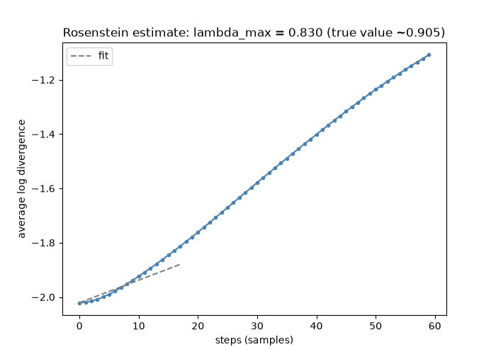
Text(0.5, 1.0, 'Rosenstein estimate: lambda_max = 0.830 (true value ~0.905)')

Is this really chaos, or just correlated noise?

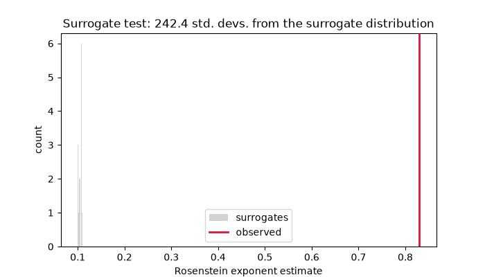
A surrogate-data test answers this rigorously: generate IAAFT surrogates (which share the series’ power spectrum and value distribution, but have randomized phases) and check whether the observed statistic is an outlier relative to them.

print("Running surrogate test (this integrates several surrogate series)...")


def statistic(series):
    return rosenstein_lyapunov(series, dim=5, tau=10, dt=dt, fit_fraction=0.3)


observed, surrogate_values, significance = surrogate_test(x, statistic, n_surrogates=19, n_iter=50, seed=0)
print(f"observed = {observed:.3f}, surrogate mean = {surrogate_values.mean():.3f}")
print(f"significance = {significance:.2f} standard deviations (>~2-3 indicates real structure)")

fig4, ax4 = plt.subplots(figsize=(7, 4))
ax4.hist(surrogate_values, bins=10, color="lightgray", label="surrogates")
ax4.axvline(observed, color="crimson", lw=2, label="observed")
ax4.set_xlabel("Rosenstein exponent estimate")
ax4.set_ylabel("count")
ax4.set_title(f"Surrogate test: {significance:.1f} std. devs. from the surrogate distribution")
ax4.legend()

Running surrogate test (this integrates several surrogate series)...
observed = 0.830, surrogate mean = 0.105
significance = 242.42 standard deviations (>~2-3 indicates real structure)

<matplotlib.legend.Legend object at 0x1368af8c0>

Spectral diagnostics

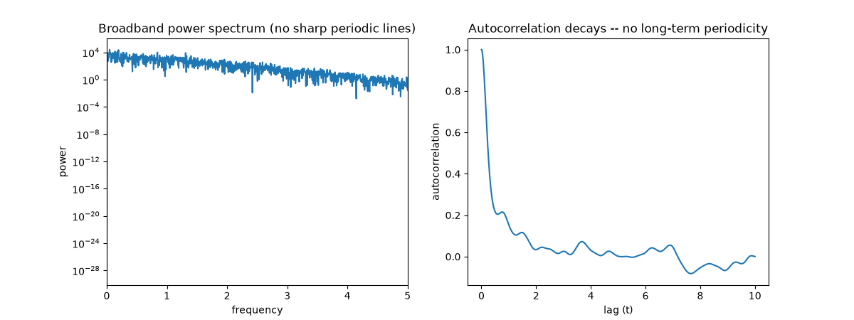
Chaos gives a broadband, continuous power spectrum – unlike a periodic or quasiperiodic signal’s sharp lines – and an autocorrelation function that decays (rather than staying periodic forever).

frequencies, power = power_spectrum(x, dt=dt)
acf = autocorrelation(x, max_lag=1000)

fig5, (ax5, ax6) = plt.subplots(1, 2, figsize=(12, 4.5))
ax5.semilogy(frequencies, power)
ax5.set_xlim(0, 5)
ax5.set_xlabel("frequency")
ax5.set_ylabel("power")
ax5.set_title("Broadband power spectrum (no sharp periodic lines)")

lags = np.arange(acf.size) * dt
ax6.plot(lags, acf)
ax6.set_xlabel("lag (t)")
ax6.set_ylabel("autocorrelation")
ax6.set_title("Autocorrelation decays -- no long-term periodicity")

plt.show()