Poincare Recurrence and Kac’s Lemma

The Poincare recurrence theorem guarantees that, for a measure-preserving system, almost every trajectory returns arbitrarily close to its starting point infinitely often. A trajectory’s recurrence structure is captured by the pairwise recurrence matrix

\[\begin{split}R_{ij} = \begin{cases} 1 & \|\mathbf{x}_i - \mathbf{x}_j\| < \epsilon \\ 0 & \text{otherwise} \end{cases}\end{split}\]

Kac’s lemma sharpens the recurrence theorem into a quantitative statement: the mean time \(\langle \tau \rangle\) between returns to a region \(A\) equals the reciprocal of that region’s invariant measure \(\mu(A)\), \(\langle \tau \rangle \approx 1/\mu(A)\). This example visualizes recurrence structure with the classic “recurrence plot” (an image of \(R_{ij}\)) for the Lorenz attractor, \(\dot{x}=\sigma(y-x)\), \(\dot{y}=x(\rho-z)-y\), \(\dot{z}=xy-\beta z\), then numerically validates Kac’s lemma on the Henon map’s attractor, \(x_{n+1}=1-ax_n^2+y_n\), \(y_{n+1}=bx_n\).

import matplotlib.pyplot as plt
import numpy as np

from physicskit.chaos.systems.continuous import Lorenz
from physicskit.chaos.systems.maps import HenonMap
from physicskit.chaos.utils.recurrence import kac_lemma_estimate
from physicskit.chaos.visualizers.recurrence import plot_recurrence_matrix, plot_recurrence_times

Recurrence plot

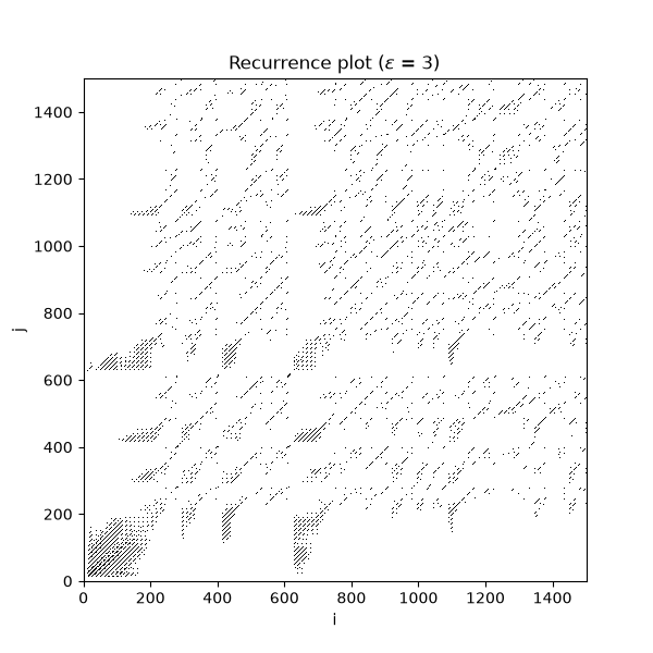
A recurrence plot marks (i, j) black whenever states i and j are within epsilon of each other. The diagonal lines and textured blocks visible here reflect the Lorenz attractor’s structure: near-diagonal bands are the smooth short-time dynamics, while the broader checkerboard pattern reflects the trajectory’s switching between the attractor’s two lobes.

lorenz = Lorenz()
_, states = lorenz.trajectory(n_steps=1500, dt=0.05)

fig, ax = plot_recurrence_matrix(states, epsilon=3.0)

Recurrence-time distribution

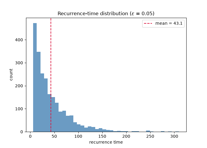
For a chaotic map, the distribution of times between successive returns to a small neighborhood is itself informative – and its mean is exactly what Kac’s lemma predicts. This example uses the Henon map, whose returns are quick to sample well (its attractor is chaotic but not fractally stretched across wildly different length scales the way Lorenz’s is).

henon = HenonMap(a=1.4, b=0.3)
traj = henon.trajectory(np.array([0.1, 0.1]), n_iter=100000)
traj = traj[500:]  # discard transient

fig2, ax2 = plot_recurrence_times(traj, epsilon=0.05, reference_idx=0)

Validating Kac’s lemma

mean_recurrence_time * measure(epsilon-ball) should be close to 1.

mean_time, measure, kac_product = kac_lemma_estimate(traj, epsilon=0.05, reference_idx=0)
print(f"mean recurrence time: {mean_time:.2f} iterations")
print(f"measure of the epsilon-ball: {measure:.5f}")
print(f"Kac's lemma product (should be close to 1): {kac_product:.4f}")

plt.show()

mean recurrence time: 43.06 iterations
measure of the epsilon-ball: 0.02321
Kac's lemma product (should be close to 1): 0.9993