Phase-Space Volume Contraction (Liouville’s Theorem)

The flow studied here is the Lorenz system,

\[\dot{x} = \sigma (y - x), \qquad \dot{y} = x (\rho - z) - y, \qquad \dot{z} = x y - \beta z.\]

Liouville’s theorem says a Hamiltonian flow preserves phase-space volume \(V\); a dissipative flow like Lorenz’s instead contracts it, according to

\[\frac{d(\log V)}{dt} = \operatorname{tr} J(x(t)),\]

where \(J\) is the flow’s Jacobian. For Lorenz, \(\operatorname{tr} J = -\sigma - 1 - \beta\) everywhere (a constant, independent of the state), so the contraction rate is exactly \(-(\sigma + 1 + \beta)\). Rather than taking that on faith from a formula, watch it happen: seed a small ball of nearby initial conditions and co-evolve every point independently – the ball visibly flattens from a sphere into a thin, wispy sheet draped over the attractor, which is both what “volume contracts” looks like and, not coincidentally, why the attractor it collapses onto is a lower-dimensional (here fractal) object rather than filling space.

import matplotlib.pyplot as plt

from physicskit.chaos.systems.continuous import Lorenz
from physicskit.chaos.utils.metrics import phase_volume_expansion
from physicskit.chaos.visualizers import animate_phase_volume_contraction

system = Lorenz(sigma=10.0, rho=28.0, beta=8.0 / 3.0)

Animation: a ball of initial conditions, collapsing

800 points, seeded in a small ball around a point already on the attractor, each integrated forward independently: watch the ball stretch into a comet-like streak within the first couple of time units, then thin out into a sparse sheet tracing both lobes of the Lorenz butterfly.

anim = animate_phase_volume_contraction(system, n_points=800, t_max=8.0, n_frames=150)

plt.show()

To save the animation to a file instead of (or in addition to) displaying it interactively, use e.g.:

anim.save("phase_volume_contraction_animation.gif", writer="pillow", fps=20)

Quantifying it: the exact contraction rate

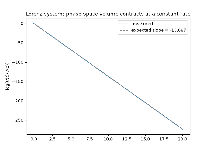
physicskit.chaos.utils.metrics.phase_volume_expansion() tracks the cumulative log phase-space volume log(V(t) / V(0)) of an infinitesimal ball co-evolved with a single reference trajectory (rather than the many finite-sized points animated above). Because the Lorenz system’s divergence is the same constant everywhere, this curve is exactly a straight line, at exactly the analytically predicted slope.

t, states = system.trajectory(n_steps=2000, dt=0.01)
log_volume = phase_volume_expansion(system, t, states)

expected_rate = -(system.sigma + 1.0 + system.beta)

fig, ax = plt.subplots(figsize=(7, 5))
ax.plot(t, log_volume, label="measured")
ax.plot(t, expected_rate * t, "--", color="gray", label=f"expected slope = {expected_rate:.3f}")
ax.set_xlabel("t")
ax.set_ylabel(r"$\log(V(t)/V(0))$")
ax.set_title("Lorenz system: phase-space volume contracts at a constant rate")
ax.legend()

plt.show()