Full Lyapunov Spectrum (Benettin QR Method)

While physicskit.chaos.visualizers.divergence.plot_lyapunov_divergence() estimates only the largest Lyapunov exponent from a single pair of trajectories, physicskit.chaos.utils.metrics.benettin_lyapunov_spectrum() estimates the full spectrum by co-evolving an orthonormal frame \(Y\) under the linearized (variational) dynamics \(\dot{Y} = J(x(t)) Y\), where \(J\) is the system’s Jacobian, and periodically re-orthonormalizing it with a QR decomposition, accumulating the log-growth of each axis. It is applied below to the Lorenz and Rossler flows,

\[\begin{split}\text{Lorenz:}\quad \dot{x} &= \sigma(y-x), & \dot{y} &= x(\rho-z)-y, & \dot{z} &= xy - \beta z \\ \text{Rossler:}\quad \dot{x} &= -y-z, & \dot{y} &= x + ay, & \dot{z} &= b + z(x-c)\end{split}\]

For a chaotic, dissipative flow like Lorenz, the spectrum has one positive exponent (chaos), one exponent near zero (the flow direction along the trajectory itself), and one strongly negative exponent (strong contraction), summing to a negative total consistent with a dissipative system. physicskit.chaos.utils.metrics.map_lyapunov_spectrum() does the same for discrete maps – demonstrated below on the dissipative Henon map, \(x_{n+1}=1-ax_n^2+y_n,\ y_{n+1}=bx_n\), and the area-preserving Chirikov-Taylor standard map, \(p_{n+1}=p_n+k\sin\theta_n \pmod{2\pi}\), \(\theta_{n+1}=\theta_n+p_{n+1}\pmod{2\pi}\).

import matplotlib.pyplot as plt
import numpy as np

from physicskit.chaos.systems.continuous import Lorenz, Rossler
from physicskit.chaos.systems.maps import HenonMap, StandardMap
from physicskit.chaos.utils.metrics import benettin_lyapunov_spectrum, map_lyapunov_spectrum

systems = {"Lorenz": Lorenz(), "Rossler": Rossler()}

Continuous flows

spectra = {name: benettin_lyapunov_spectrum(system, system.initial_state(), dt=0.01, n_steps=8000, n_transient=1000) for name, system in systems.items()}
for name, spectrum in spectra.items():
    print(f"{name} Lyapunov spectrum: {spectrum} (sum = {spectrum.sum():.3f})")

fig, ax = plt.subplots(figsize=(7, 5))
width = 0.35
for offset, (name, spectrum) in zip((-width / 2, width / 2), spectra.items()):
    idx = np.arange(len(spectrum)) + offset
    ax.bar(idx, spectrum, width=width, label=name)
ax.axhline(0.0, color="black", lw=0.8)
ax.set_xticks(range(3))
ax.set_xticklabels([r"$\lambda_1$", r"$\lambda_2$", r"$\lambda_3$"])
ax.set_ylabel("Lyapunov exponent")
ax.set_title("Lyapunov spectra: Lorenz vs. Rossler")
ax.legend()

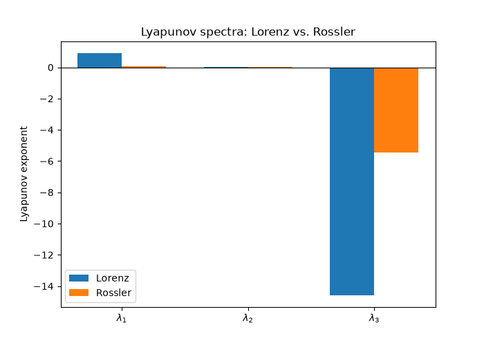
Lorenz Lyapunov spectrum: [  0.88601347   0.01735502 -14.56993363] (sum = -13.667)
Rossler Lyapunov spectrum: [ 0.07105687  0.00997877 -5.43497703] (sum = -5.354)

<matplotlib.legend.Legend object at 0x136adaf90>

Discrete maps

The same Benettin QR method applies to discrete maps, just without a dt to divide by. As a check on the estimate’s quality: the Henon map’s Jacobian determinant is exactly -b everywhere, so its spectrum must sum to exactly ln|b|; the standard map is exactly area-preserving, so its spectrum must sum to exactly zero – both hold regardless of how precisely the individual exponents are estimated.

henon = HenonMap(a=1.4, b=0.3)
standard = StandardMap(k=2.0)
henon_spectrum = map_lyapunov_spectrum(henon, henon.initial_state(), n_iter=10000, n_transient=1000)
standard_spectrum = map_lyapunov_spectrum(standard, standard.initial_state(), n_iter=10000, n_transient=1000)
print(f"Henon spectrum: {henon_spectrum} (sum = {henon_spectrum.sum():.4f}, ln|b| = {np.log(0.3):.4f})")
print(f"Standard map spectrum: {standard_spectrum} (sum = {standard_spectrum.sum():.4f})")

fig2, ax2 = plt.subplots(figsize=(6, 5))
width = 0.35
for offset, (name, spectrum) in zip((-width / 2, width / 2), [("Henon", henon_spectrum), ("Standard map", standard_spectrum)]):
    idx = np.arange(len(spectrum)) + offset
    ax2.bar(idx, spectrum, width=width, label=name)
ax2.axhline(0.0, color="black", lw=0.8)
ax2.set_xticks(range(2))
ax2.set_xticklabels([r"$\lambda_1$", r"$\lambda_2$"])
ax2.set_ylabel("Lyapunov exponent (per iteration)")
ax2.set_title("Lyapunov spectra: Henon (dissipative) vs. Standard map (conservative)")
ax2.legend()

plt.show()

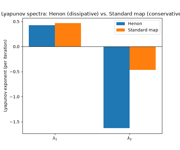
Henon spectrum: [ 0.42652047 -1.63049328] (sum = -1.2040, ln|b| = -1.2040)
Standard map spectrum: [ 0.46525272 -0.46525272] (sum = 0.0000)