Lyapunov Divergence: Chaotic vs. Non-Chaotic

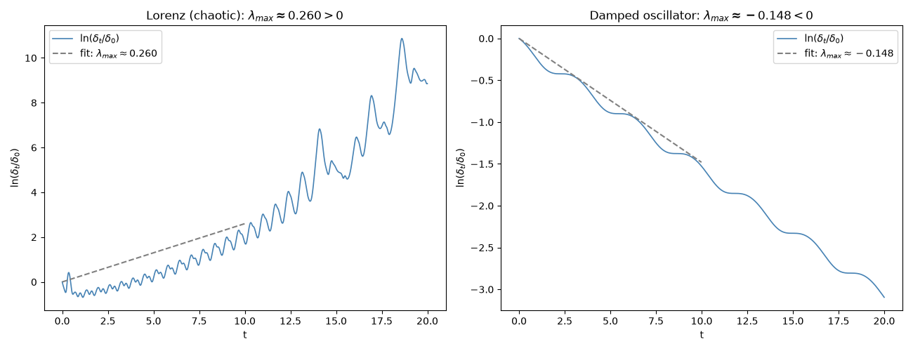
physicskit.chaos.visualizers.divergence.plot_lyapunov_divergence() integrates two trajectories starting an infinitesimal distance \(\delta_0\) apart and tracks \(\ln(\delta_t / \delta_0)\) over time, where \(\delta_t\) is their separation at time \(t\). For chaotic motion this separation grows exponentially, \(\delta_t \sim \delta_0 e^{\lambda_{\max} t}\), so a straight, positively-sloped line (its slope the largest Lyapunov exponent \(\lambda_{\max} > 0\)) is the signature of chaos; a system that is not chaotic instead shows the separation shrinking (\(\lambda_{\max} < 0\)) as both trajectories relax toward the same attracting state. Two systems are contrasted below: the chaotic Lorenz attractor, \(\dot{x}=\sigma(y-x)\), \(\dot{y}=x(\rho-z)-y\), \(\dot{z}=xy-\beta z\); and the Duffing oscillator, \(\ddot{x}+\delta_D \dot{x}+\alpha x+\beta_D x^3=\gamma\cos(\omega t)\), with its cubic term and forcing switched off (\(\beta_D=\gamma=0\), \(\alpha=1 > 0\)), which reduces it to a plain damped linear oscillator, \(\ddot{x}+\delta_D \dot{x}+x=0\): every trajectory relaxes to the same fixed point, so nearby trajectories converge rather than diverge.

import matplotlib.pyplot as plt

from physicskit.chaos.systems.continuous import Duffing, Lorenz
from physicskit.chaos.visualizers.divergence import plot_lyapunov_divergence

Chaotic case: Lorenz

lorenz = Lorenz()

Non-chaotic case: an undriven, damped (linear) oscillator

Setting the Duffing oscillator’s forcing amplitude to zero and its cubic term to zero leaves a plain damped harmonic oscillator: every trajectory relaxes to the same fixed point, so nearby trajectories converge rather than diverge.

damped = Duffing(delta=0.3, alpha=1.0, beta=0.0, gamma=0.0, omega=1.0)

fig, (ax1, ax2) = plt.subplots(1, 2, figsize=(13, 5))
_, _, lam_lorenz = plot_lyapunov_divergence(lorenz, t_max=20.0, n_points=1000, ax=ax1, seed=0)
_, _, lam_damped = plot_lyapunov_divergence(damped, t_max=20.0, n_points=1000, ax=ax2, seed=0)
ax1.set_title(f"Lorenz (chaotic): $\\lambda_{{max}} \\approx {lam_lorenz:.3f} > 0$")
ax2.set_title(f"Damped oscillator: $\\lambda_{{max}} \\approx {lam_damped:.3f} < 0$")
fig.tight_layout()

plt.show()