Pomeau-Manneville intermittency: laminar phases and chaotic bursts

Pomeau and Manneville (1980) identified a third route to chaos, distinct from period-doubling and quasi-periodicity: near a tangent (saddle-node) bifurcation, a trajectory spends increasingly long, apparently regular “laminar” episodes near the fixed point about to vanish, each interrupted by a short chaotic burst, with the mean laminar length diverging as a power law as the tangency is approached. LogisticMap’s period-three window is born at exactly such a tangent bifurcation, at \(r\approx3.8284\); this example iterates the map at values of \(r\) just below that threshold and shows both halves of the phenomenon directly: the laminar-then-burst time series itself, and the mean laminar length growing as \(r\) approaches the tangency.

import matplotlib.pyplot as plt
import numpy as np

from physicskit.chaos.systems.maps import LogisticMap

The laminar-burst time series

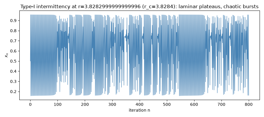
Just below the period-three window’s tangent bifurcation, the trajectory spends long stretches shadowing an (almost) period-3 orbit – laminar phases – each abruptly ended by a short chaotic burst that reinjects it, before the next laminar episode begins.

r_c = 3.8284  # the period-3 window's tangent-bifurcation threshold
r = r_c - 1e-4

m = LogisticMap(r=r)
n_iter = 800
traj = m.trajectory(np.array([0.5]), n_iter=n_iter).flatten()

fig1, ax1 = plt.subplots(figsize=(9, 4))
ax1.plot(traj, color="steelblue", lw=0.9)
ax1.set_xlabel("iteration n")
ax1.set_ylabel(r"$x_n$")
ax1.set_title(f"Type-I intermittency at r={r} (r_c={r_c}): laminar plateaus, chaotic bursts")
fig1.tight_layout()

Detecting laminar episodes directly

A period-3 laminar phase means x_n stays close to x_{n-3}; comparing every point to the one three iterations earlier isolates exactly the near-periodic stretches from the chaotic bursts between them.

tol = 0.01


def laminar_run_lengths(r_value, n_iter=30_000, tol=tol):
    traj = LogisticMap(r=r_value).trajectory(np.array([0.5]), n_iter=n_iter).flatten()
    is_laminar = np.abs(traj[3:] - traj[:-3]) < tol
    runs, count = [], 0
    for v in is_laminar:
        if v:
            count += 1
        else:
            if count > 0:
                runs.append(count)
            count = 0
    if count > 0:
        runs.append(count)
    return np.array(runs)


runs = laminar_run_lengths(r)
print(f"at r={r} (r_c - r = {r_c - r:.1e}): {len(runs)} laminar episodes found")
print(f"laminar run lengths (first 15): {runs[:15]}")
print(f"mean laminar length: {runs.mean():.2f}")

at r=3.8282999999999996 (r_c - r = 1.0e-04): 926 laminar episodes found
laminar run lengths (first 15): [90  1  6  1 17  1 24  1 24  1  1  2  1  1  2]
mean laminar length: 19.91

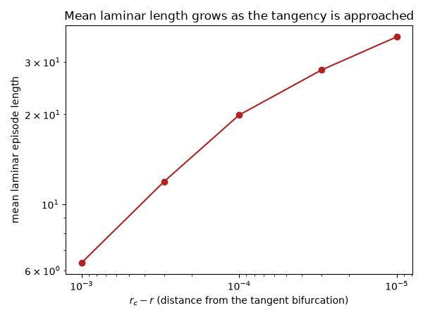
Mean laminar length diverges as the tangency is approached

distances = np.array([1e-3, 3e-4, 1e-4, 3e-5, 1e-5])
mean_lengths = np.array([laminar_run_lengths(r_c - d).mean() for d in distances])

print("\nr_c - r        mean laminar length")
for d, ell in zip(distances, mean_lengths):
    print(f"  {d:.1e}        {ell:8.2f}")

fig2, ax2 = plt.subplots(figsize=(6, 4.5))
ax2.loglog(distances, mean_lengths, "o-", color="firebrick")
ax2.set_xlabel(r"$r_c - r$ (distance from the tangent bifurcation)")
ax2.set_ylabel("mean laminar episode length")
ax2.set_title("Mean laminar length grows as the tangency is approached")
ax2.invert_xaxis()
fig2.tight_layout()

plt.show()

r_c - r        mean laminar length
  1.0e-03            6.36
  3.0e-04           11.90
  1.0e-04           19.91
  3.0e-05           28.19
  1.0e-05           36.40