Fractal Dimension: Box-Counting and Correlation Dimension

Strange attractors are fractals: their box-counting (capacity) dimension \(D_0\) and correlation dimension \(D_2\) are non-integers, quantifying how densely (or sparsely) the attractor fills the space it lives in. Covering the attractor with boxes of side \(\epsilon\) and counting the occupied boxes \(N(\epsilon)\),

\[D_0 = \lim_{\epsilon \to 0} \frac{\log N(\epsilon)}{\log(1/\epsilon)},\]

estimated here as the slope of \(\log N(\epsilon)\) vs. \(\log(1/\epsilon)\). The correlation dimension instead uses the fraction \(C(\epsilon)\) of all point pairs closer than \(\epsilon\),

\[D_2 = \lim_{\epsilon \to 0} \frac{\log C(\epsilon)}{\log \epsilon},\]

estimated as the slope of \(\log C(\epsilon)\) vs. \(\log\epsilon\) (the Grassberger-Procaccia algorithm). This example first validates both estimators against the middle-thirds Cantor set, whose dimension is known exactly in closed form (\(\log 2 / \log 3 \approx 0.631\)), then applies them to the strange attractor of the Henon map, \(x_{n+1} = 1 - a x_n^2 + y_n,\ y_{n+1} = b x_n\) with the classic chaotic parameters \(a=1.4\), \(b=0.3\).

import matplotlib.pyplot as plt
import numpy as np

from physicskit.chaos.systems.maps import HenonMap
from physicskit.chaos.utils.dimension import box_counting_dimension, correlation_dimension

Ground truth: the Cantor set

The middle-thirds Cantor set has an exactly known dimension, log(2)/log(3) ~= 0.631, making it the standard sanity check for any fractal-dimension estimator.

def cantor_set_points(n_iter=10):
    intervals = [(0.0, 1.0)]
    for _ in range(n_iter):
        intervals = [piece for a, b in intervals for piece in ((a, a + (b - a) / 3.0), (b - (b - a) / 3.0, b))]
    return np.array([[(a + b) / 2.0] for a, b in intervals])


cantor_points = cantor_set_points(n_iter=10)
cantor_dimension = np.log(2) / np.log(3)

d0_cantor, eps0, counts0 = box_counting_dimension(cantor_points, n_scales=15, eps_min=3.0**-8, eps_max=3.0**-2)
d2_cantor, eps2, csum2 = correlation_dimension(cantor_points, n_scales=15, eps_min=3.0**-8, eps_max=3.0**-2)
print(f"Cantor set: exact dimension = {cantor_dimension:.4f}")
print(f"  box-counting estimate D0 = {d0_cantor:.4f}")
print(f"  correlation estimate  D2 = {d2_cantor:.4f}")

fig, axes = plt.subplots(1, 2, figsize=(12, 5))
axes[0].loglog(1.0 / eps0, counts0, "o-")
axes[0].set_xlabel(r"$1/\epsilon$")
axes[0].set_ylabel(r"$N(\epsilon)$")
axes[0].set_title(f"Box counting: D0 = {d0_cantor:.3f} (exact: {cantor_dimension:.3f})")

axes[1].loglog(eps2, csum2, "o-", color="darkorange")
axes[1].set_xlabel(r"$\epsilon$")
axes[1].set_ylabel(r"$C(\epsilon)$")
axes[1].set_title(f"Correlation sum: D2 = {d2_cantor:.3f} (exact: {cantor_dimension:.3f})")
fig.suptitle("Validating both estimators against the Cantor set")
fig.tight_layout()

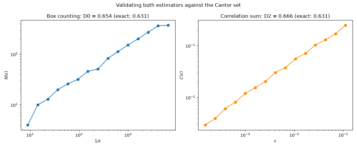
Cantor set: exact dimension = 0.6309
  box-counting estimate D0 = 0.6541
  correlation estimate  D2 = 0.6657

The Henon attractor

The classic Henon attractor (a=1.4, b=0.3) has a well-documented fractal dimension of approximately 1.2-1.3 – between a curve (dimension 1) and a filled region (dimension 2), reflecting its densely-layered, sheet-like fractal structure.

henon = HenonMap(a=1.4, b=0.3)
traj = henon.trajectory(np.array([0.0, 0.0]), n_iter=8000)
traj = traj[500:]  # discard transient

d0_henon, eps0h, counts0h = box_counting_dimension(traj)
d2_henon, eps2h, csum2h = correlation_dimension(traj)
print(f"Henon attractor: box-counting D0 = {d0_henon:.4f}, correlation D2 = {d2_henon:.4f}")

fig2, ax2 = plt.subplots(figsize=(6, 6))
ax2.scatter(traj[:, 0], traj[:, 1], s=0.3, color="darkgreen", alpha=0.5)
ax2.set_title(f"Henon attractor (D0 = {d0_henon:.2f}, D2 = {d2_henon:.2f})")

plt.show()

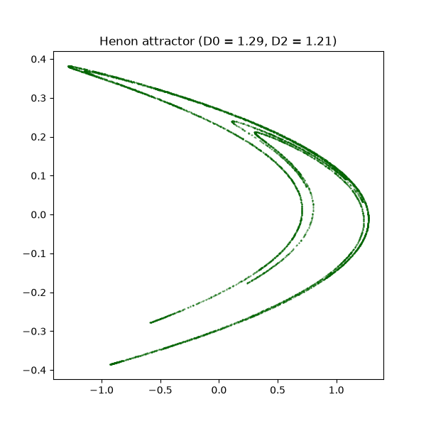
Henon attractor: box-counting D0 = 1.2935, correlation D2 = 1.2096