Energy Drift vs. Integration Step Size

physicskit.chaos.utils.metrics.energy_drift() measures how well a numerical integrator conserves a system’s total energy. The system here is the planar double pendulum – point masses \(m_1\), \(m_2\) on massless rods of length \(l_1\), \(l_2\), hanging under gravity \(g\) – whose total mechanical energy in terms of the rod angles \(\theta_1, \theta_2\) and angular velocities \(\omega_1, \omega_2\) is

\[E = \underbrace{\tfrac{1}{2}m_1 (l_1 \omega_1)^2 + \tfrac{1}{2}m_2 \left[(l_1\omega_1)^2 + (l_2\omega_2)^2 + 2 l_1 l_2 \omega_1 \omega_2 \cos(\theta_1 - \theta_2)\right]}_{\text{kinetic}} \underbrace{- (m_1+m_2) g l_1 \cos\theta_1 - m_2 g l_2 \cos\theta_2}_{\text{potential}}.\]

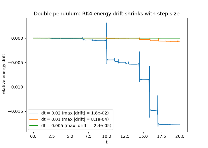
Since the double pendulum is conservative but RK4 is not exactly energy-preserving, the residual drift in \(E\) along a numerically integrated trajectory is purely numerical error – and it should shrink rapidly as the step size dt is refined, since RK4 has 4th-order local accuracy. 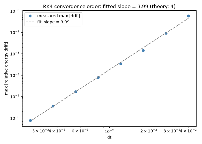This example integrates the same physical trajectory at three different step sizes and compares the resulting drift, then checks that “4th-order” claim directly: sweeping dt over a wider range and plotting the worst-case drift on log-log axes against a fitted power law recovers a slope close to the theoretical 4.

import matplotlib.pyplot as plt
import numpy as np

from physicskit.chaos.systems.continuous import DoublePendulum
from physicskit.chaos.utils.metrics import energy_drift

system = DoublePendulum()
state0 = np.array([np.pi / 2, np.pi / 2, 0.0, 0.0])
t_max = 20.0

Integrate at several step sizes

fig, ax = plt.subplots(figsize=(7, 5))
for dt in (0.02, 0.01, 0.005):
    n_steps = int(t_max / dt)
    t, states = system.trajectory(state0=state0, dt=dt, n_steps=n_steps)
    drift = energy_drift(t, states, system.energy)
    ax.plot(t, drift, label=f"dt = {dt} (max |drift| = {np.max(np.abs(drift)):.1e})")

ax.set_xlabel("t")
ax.set_ylabel("relative energy drift")
ax.set_title("Double pendulum: RK4 energy drift shrinks with step size")
ax.legend()

<matplotlib.legend.Legend object at 0x1508cf560>

Checking the “4th order” claim: worst-case drift vs. step size

RK4’s local truncation error is \(O(dt^5)\) per step, which accumulates to a global error of \(O(dt^4)\) over a fixed integration time – so the worst-case energy drift should fall off as \(dt^4\) as dt shrinks. A wider, finer sweep of step sizes (over a much shorter integration window, since only the local scaling behavior is needed here, not the drift’s time-dependence already shown above) puts that scaling to the test: fitting a line to log(max drift) vs. log(dt) should recover a slope close to the theoretical value of 4.

dt_values = np.geomspace(0.04, 0.0025, 8)
max_drift = np.empty_like(dt_values)
for i, dt_i in enumerate(dt_values):
    n_steps_i = int(round(2.0 / dt_i))
    t_i, states_i = system.trajectory(state0=state0, dt=dt_i, n_steps=n_steps_i)
    max_drift[i] = np.max(np.abs(energy_drift(t_i, states_i, system.energy)))

slope, intercept = np.polyfit(np.log(dt_values), np.log(max_drift), 1)

fig2, ax2 = plt.subplots(figsize=(7, 5))
ax2.loglog(dt_values, max_drift, "o", color="steelblue", label="measured max |drift|")
ax2.loglog(dt_values, np.exp(intercept) * dt_values**slope, "--", color="gray", label=f"fit: slope = {slope:.2f}")
ax2.set_xlabel("dt")
ax2.set_ylabel("max |relative energy drift|")
ax2.set_title(f"RK4 convergence order: fitted slope = {slope:.2f} (theory: 4)")
ax2.legend()
fig2.tight_layout()

plt.show()