Bifurcation Diagrams for Continuous Flows: the Duffing Oscillator

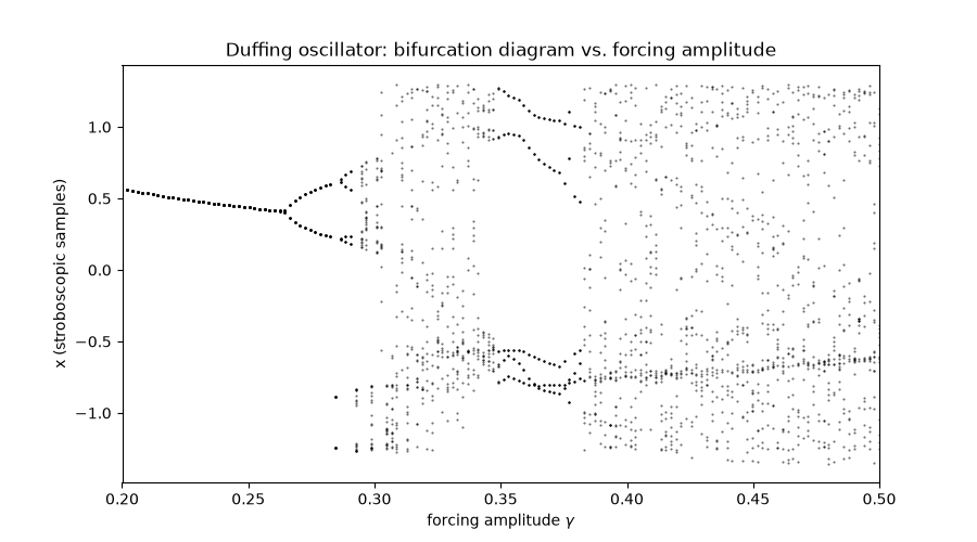
Bifurcation diagrams aren’t only for discrete maps – they’re just as useful for continuous, periodically-forced flows, via a stroboscopic Poincare section: sampling the state once per forcing period turns the continuous flow into an effective discrete map. The flow swept here is the forced, damped Duffing oscillator,

\[\ddot{x} + \delta \dot{x} + \alpha x + \beta x^3 = \gamma \cos(\omega t),\]

with fixed damping \(\delta=0.3\), linear stiffness \(\alpha=-1\), cubic stiffness \(\beta=1\), and forcing frequency \(\omega=1.2\) (so the double-well potential and forcing frequency are held fixed while only the forcing amplitude \(\gamma\) is swept). This example sweeps \(\gamma\) and, for each value, plots the surviving stroboscopic samples, using physicskit.chaos.visualizers.bifurcation.stroboscopic_bifurcation_sampler() – the same plot_bifurcation_diagram() used for the Logistic Map works here completely unchanged. A companion plot below sweeps the same \(\gamma\) range with physicskit.chaos.visualizers.divergence.trajectory_divergence() and physicskit.chaos.utils.metrics.lyapunov_exponent_from_divergence() to estimate the largest Lyapunov exponent at each amplitude, turning the bifurcation diagram’s purely qualitative “band looks chaotic” into the quantitative \(\lambda_{\max} > 0\) criterion, on the same \(\gamma\) axis.

import matplotlib.pyplot as plt
import numpy as np

from physicskit.chaos.systems.continuous import Duffing
from physicskit.chaos.utils.metrics import lyapunov_exponent_from_divergence
from physicskit.chaos.visualizers.bifurcation import (
    plot_bifurcation_diagram,
    stroboscopic_bifurcation_sampler,
)
from physicskit.chaos.visualizers.divergence import trajectory_divergence

Build the stroboscopic sampler

The forcing period is 2*pi / omega; sampling the state once per forcing period is what turns the continuous flow into an effective discrete map.

omega = 1.2
period = 2.0 * np.pi / omega

sampler = stroboscopic_bifurcation_sampler(
    lambda gamma: Duffing(delta=0.3, alpha=-1.0, beta=1.0, gamma=gamma, omega=omega),
    state0=np.array([0.1, 0.0]),
    sample_period=period,
    n_transient_periods=60,
    n_keep_periods=20,
    component=0,
    dt=0.15,
    rtol=1e-6,
    atol=1e-8,
)

Sweep the forcing amplitude

As gamma increases, watch the single-point regular response give way to period-doubled cycles, and eventually a chaotic band – the same period-doubling route to chaos as the Logistic Map, now in a physically driven mechanical oscillator. (Looser tolerances than the sampler’s defaults keep this parameter sweep fast – it calls the integrator once per gamma value below.) Each gamma value is fully independent of every other, so this sweep is also embarrassingly parallel: n_jobs runs it across a thread pool (real speedup here, since solve_ivp releases the GIL while it integrates), and show_progress displays a tqdm bar.

gamma_values = np.linspace(0.2, 0.5, 150)
fig, ax = plt.subplots(figsize=(9, 5))
plot_bifurcation_diagram(gamma_values, sampler, n_jobs=4, show_progress=True, marker=".", markersize=1.0, ax=ax)
ax.set_xlabel(r"forcing amplitude $\gamma$")
ax.set_ylabel("x (stroboscopic samples)")
ax.set_title("Duffing oscillator: bifurcation diagram vs. forcing amplitude")

plt.show()

sweeping:   0%|          | 0/150 [00:00<?, ?it/s]
sweeping:   1%|          | 1/150 [00:00<01:18,  1.90it/s]
sweeping:   3%|▎         | 5/150 [00:00<00:19,  7.41it/s]
sweeping:   4%|▍         | 6/150 [00:00<00:19,  7.39it/s]
sweeping:   5%|▌         | 8/150 [00:01<00:17,  7.96it/s]
sweeping:   7%|▋         | 10/150 [00:01<00:17,  8.21it/s]
sweeping:   7%|▋         | 11/150 [00:01<00:17,  8.13it/s]
sweeping:   8%|▊         | 12/150 [00:01<00:17,  7.78it/s]
sweeping:   9%|▉         | 14/150 [00:01<00:15,  8.87it/s]
sweeping:  10%|█         | 15/150 [00:02<00:17,  7.87it/s]
sweeping:  11%|█▏        | 17/150 [00:02<00:14,  8.94it/s]
sweeping:  13%|█▎        | 19/150 [00:02<00:13,  9.56it/s]
sweeping:  13%|█▎        | 20/150 [00:02<00:14,  9.03it/s]
sweeping:  14%|█▍        | 21/150 [00:02<00:16,  7.67it/s]
sweeping:  16%|█▌        | 24/150 [00:03<00:15,  8.32it/s]
sweeping:  17%|█▋        | 25/150 [00:03<00:16,  7.46it/s]
sweeping:  19%|█▊        | 28/150 [00:03<00:14,  8.19it/s]
sweeping:  21%|██        | 31/150 [00:03<00:11, 10.40it/s]
sweeping:  22%|██▏       | 33/150 [00:04<00:13,  8.63it/s]
sweeping:  23%|██▎       | 35/150 [00:04<00:12,  9.00it/s]
sweeping:  25%|██▍       | 37/150 [00:04<00:13,  8.16it/s]
sweeping:  26%|██▌       | 39/150 [00:04<00:13,  8.12it/s]
sweeping:  27%|██▋       | 41/150 [00:04<00:11,  9.29it/s]
sweeping:  29%|██▊       | 43/150 [00:05<00:09, 10.75it/s]
sweeping:  30%|███       | 45/150 [00:05<00:12,  8.57it/s]
sweeping:  31%|███▏      | 47/150 [00:05<00:10, 10.26it/s]
sweeping:  33%|███▎      | 49/150 [00:05<00:12,  8.29it/s]
sweeping:  34%|███▍      | 51/150 [00:05<00:10,  9.49it/s]
sweeping:  35%|███▌      | 53/150 [00:06<00:10,  8.94it/s]
sweeping:  37%|███▋      | 55/150 [00:06<00:10,  8.65it/s]
sweeping:  38%|███▊      | 57/150 [00:06<00:10,  8.86it/s]
sweeping:  39%|███▊      | 58/150 [00:06<00:10,  8.41it/s]
sweeping:  39%|███▉      | 59/150 [00:06<00:11,  8.11it/s]
sweeping:  41%|████      | 61/150 [00:07<00:09,  9.68it/s]
sweeping:  42%|████▏     | 63/150 [00:07<00:09,  9.43it/s]
sweeping:  43%|████▎     | 64/150 [00:07<00:09,  9.12it/s]
sweeping:  43%|████▎     | 65/150 [00:07<00:09,  9.21it/s]
sweeping:  45%|████▍     | 67/150 [00:07<00:09,  8.64it/s]
sweeping:  45%|████▌     | 68/150 [00:07<00:09,  8.33it/s]
sweeping:  47%|████▋     | 71/150 [00:08<00:09,  8.30it/s]
sweeping:  48%|████▊     | 72/150 [00:08<00:09,  8.18it/s]
sweeping:  50%|█████     | 75/150 [00:08<00:08,  8.71it/s]
sweeping:  51%|█████▏    | 77/150 [00:08<00:07, 10.34it/s]
sweeping:  53%|█████▎    | 79/150 [00:09<00:09,  7.71it/s]
sweeping:  55%|█████▍    | 82/150 [00:09<00:06,  9.87it/s]
sweeping:  56%|█████▌    | 84/150 [00:09<00:07,  8.65it/s]
sweeping:  57%|█████▋    | 86/150 [00:10<00:07,  8.84it/s]
sweeping:  59%|█████▊    | 88/150 [00:10<00:07,  8.31it/s]
sweeping:  61%|██████    | 91/150 [00:10<00:06,  9.41it/s]
sweeping:  62%|██████▏   | 93/150 [00:10<00:06,  8.68it/s]
sweeping:  63%|██████▎   | 95/150 [00:10<00:05,  9.57it/s]
sweeping:  65%|██████▍   | 97/150 [00:11<00:05,  9.24it/s]
sweeping:  65%|██████▌   | 98/150 [00:11<00:05,  9.21it/s]
sweeping:  66%|██████▌   | 99/150 [00:11<00:05,  8.52it/s]
sweeping:  67%|██████▋   | 101/150 [00:11<00:05,  9.48it/s]
sweeping:  68%|██████▊   | 102/150 [00:11<00:05,  8.02it/s]
sweeping:  69%|██████▉   | 104/150 [00:11<00:04,  9.68it/s]
sweeping:  71%|███████   | 106/150 [00:12<00:04,  9.35it/s]
sweeping:  71%|███████▏  | 107/150 [00:12<00:05,  8.27it/s]
sweeping:  73%|███████▎  | 109/150 [00:12<00:04,  9.27it/s]
sweeping:  74%|███████▍  | 111/150 [00:12<00:05,  7.80it/s]
sweeping:  75%|███████▌  | 113/150 [00:12<00:03,  9.51it/s]
sweeping:  77%|███████▋  | 115/150 [00:13<00:04,  7.63it/s]
sweeping:  79%|███████▉  | 119/150 [00:13<00:03,  9.20it/s]
sweeping:  81%|████████  | 121/150 [00:13<00:02,  9.85it/s]
sweeping:  82%|████████▏ | 123/150 [00:14<00:02,  9.50it/s]
sweeping:  83%|████████▎ | 125/150 [00:14<00:02,  9.28it/s]
sweeping:  84%|████████▍ | 126/150 [00:14<00:02,  9.03it/s]
sweeping:  85%|████████▌ | 128/150 [00:14<00:02,  7.46it/s]
sweeping:  87%|████████▋ | 130/150 [00:14<00:02,  8.67it/s]
sweeping:  88%|████████▊ | 132/150 [00:15<00:02,  8.64it/s]
sweeping:  89%|████████▊ | 133/150 [00:15<00:01,  8.52it/s]
sweeping:  90%|█████████ | 135/150 [00:15<00:01, 10.15it/s]
sweeping:  91%|█████████▏| 137/150 [00:15<00:01, 10.37it/s]
sweeping:  93%|█████████▎| 139/150 [00:15<00:01,  8.62it/s]
sweeping:  94%|█████████▍| 141/150 [00:16<00:00,  9.93it/s]
sweeping:  95%|█████████▌| 143/150 [00:16<00:00,  7.60it/s]
sweeping:  97%|█████████▋| 146/150 [00:16<00:00,  7.69it/s]
sweeping: 100%|██████████| 150/150 [00:16<00:00,  8.84it/s]

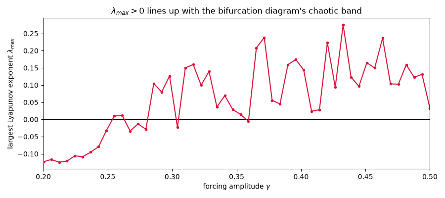
Quantifying it: the largest Lyapunov exponent, on the same axis

The bifurcation diagram above only shows where the response looks irregular; it doesn’t say whether that irregularity is genuine exponential sensitivity or “just” a very long periodic cycle. Sweeping the same gamma_values (on a coarser grid, since each point here integrates two whole trajectories rather than sampling one) with trajectory_divergence() and fitting the growth rate of two initially nearby trajectories’ separation gives the largest Lyapunov exponent \(\lambda_{\max}\) directly: it should track the bifurcation diagram closely, crossing zero right around where the single point (or handful of stroboscopic points) gives way to the dense chaotic band above.

gamma_values_lyap = np.linspace(0.2, 0.5, 50)
lyapunov_exponents = np.empty_like(gamma_values_lyap)
for i, gamma in enumerate(gamma_values_lyap):
    lyap_system = Duffing(delta=0.3, alpha=-1.0, beta=1.0, gamma=float(gamma), omega=omega)
    t_div, delta_t = trajectory_divergence(lyap_system, state0=np.array([0.1, 0.0]), delta_0=1e-8, t_max=150.0, n_points=400, seed=0)
    n_fit = int(0.5 * t_div.size)
    lyapunov_exponents[i] = lyapunov_exponent_from_divergence(t_div[:n_fit], delta_t[:n_fit] / 1e-8)

fig_lyap, ax_lyap = plt.subplots(figsize=(9, 4))
ax_lyap.axhline(0.0, color="black", lw=0.8)
ax_lyap.plot(gamma_values_lyap, lyapunov_exponents, "o-", color="crimson", markersize=3)
ax_lyap.set_xlim(gamma_values[0], gamma_values[-1])
ax_lyap.set_xlabel(r"forcing amplitude $\gamma$")
ax_lyap.set_ylabel(r"largest Lyapunov exponent $\lambda_{max}$")
ax_lyap.set_title(r"$\lambda_{max} > 0$ lines up with the bifurcation diagram's chaotic band")
fig_lyap.tight_layout()

plt.show()