Logistic Map: the Period-Doubling Route to Chaos

The logistic map,

\[x_{n+1} = r x_n (1 - x_n),\]

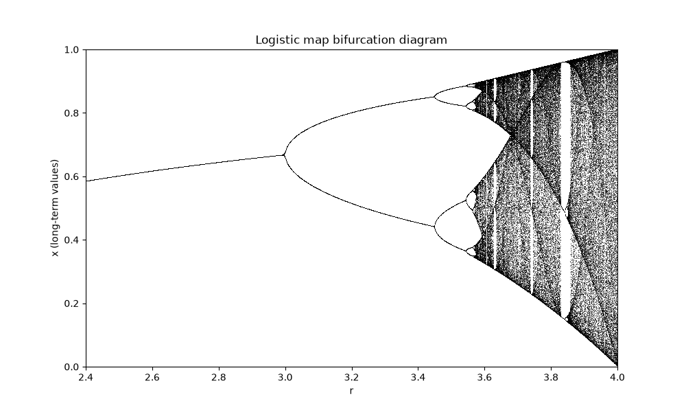
is the simplest possible model of the period-doubling cascade: as the single growth-rate parameter \(r\) is increased over \([0, 4]\), a stable fixed point splits into a stable 2-cycle, then a 4-cycle, then 8, 16, … with the bifurcations arriving at an ever-shrinking rate that converges geometrically to the universal Feigenbaum constant \(\delta \approx 4.669\), accumulating at \(r \approx 3.5699\) onto the onset of chaos. Beyond that value the map is chaotic for most (but not all – note the periodic windows, the largest starting near \(r \approx 3.8284\)) values of \(r\) up to \(r=4\); the example below uses \(r=3.9\), deep in the chaotic regime.

import matplotlib.pyplot as plt
import numpy as np

from physicskit.chaos.systems.maps import LogisticMap
from physicskit.chaos.visualizers.bifurcation import map_bifurcation_sampler, plot_bifurcation_diagram
from physicskit.chaos.visualizers.dynamic_plots import animate_map_cobweb

system = LogisticMap(r=3.9)

Animation: the cobweb diagram

The classic way to see a 1D map’s dynamics geometrically: bounce between the map curve f(x) (vertical jumps, computing the next value) and the diagonal y = x (horizontal jumps, feeding that value back in). For r=3.9 the orbit never settles down – the cobweb keeps exploring new territory instead of converging onto a fixed point or a short cycle.

anim = animate_map_cobweb(system, x0=0.4, n_iter=40)

plt.show()

To save the animation to a file instead of (or in addition to) displaying it interactively, use e.g.:

anim.save("logistic_map_animation.gif", writer="pillow", fps=5)

A single chaotic trajectory

traj = system.trajectory(np.array([0.4]), n_iter=200)

fig, ax = plt.subplots(figsize=(8, 4))
ax.plot(traj[:, 0], lw=1.0, marker=".", markersize=3)
ax.set_xlabel("iteration n")
ax.set_ylabel("x")
ax.set_title(f"Logistic map trajectory, r = {system.r}")

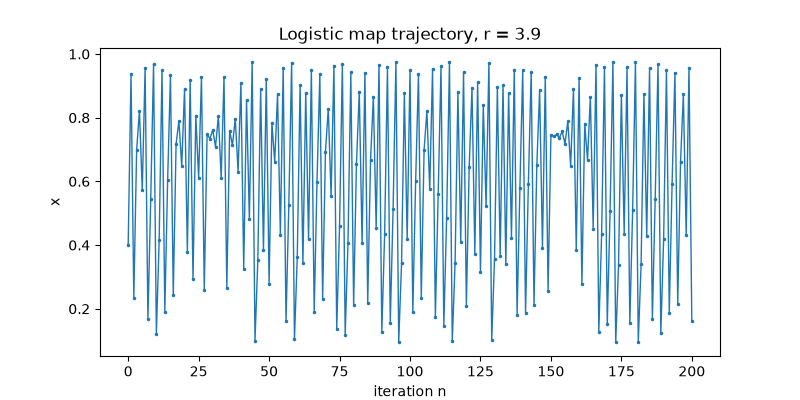
Text(0.5, 1.0, 'Logistic map trajectory, r = 3.9')

The bifurcation diagram

physicskit.chaos.visualizers.bifurcation.plot_bifurcation_diagram() sweeps r, iterating each map instance past its transient and plotting the surviving long-term values: a single point for a fixed point, a handful of points for a period-k cycle, and a dense band for chaos. This is the single image most associated with “the route to chaos”.

r_values = np.linspace(2.4, 4.0, 2000)
sampler = map_bifurcation_sampler(lambda r: LogisticMap(r=r), state0=np.array([0.5]), n_transient=500, n_keep=200)

fig2, ax2 = plot_bifurcation_diagram(r_values, sampler)
ax2.set_xlabel("r")
ax2.set_ylabel("x (long-term values)")
ax2.set_title("Logistic map bifurcation diagram")
ax2.set_ylim(0.0, 1.0)

plt.show()