Smale’s Horseshoe Map: Stretch, Fold, and Return

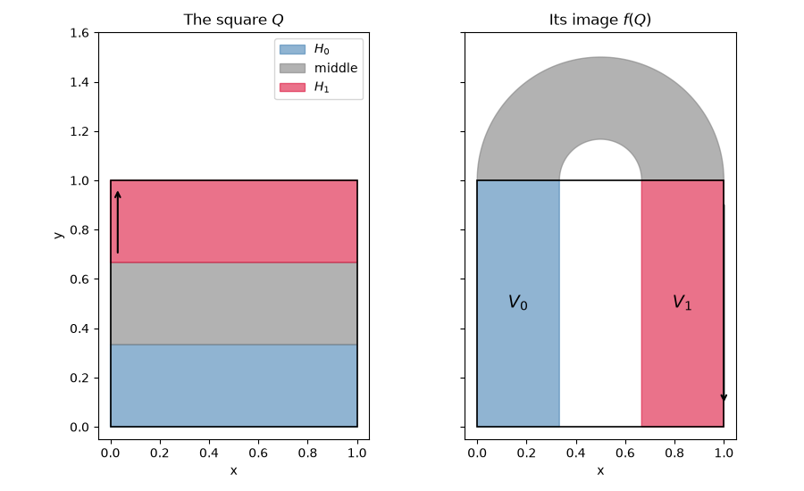
Smale’s horseshoe (1965) takes the unit square \(Q\), squeezes it horizontally by \(\lambda < 1/2\), stretches it vertically by \(\mu > 2\), and bends the resulting strip into a U whose two legs lie back across \(Q\). Only two horizontal strips of the square return to it, each by an affine branch:

\[\begin{split}f(x, y) = \begin{cases} (\lambda x,\ \mu y) & y \le 1/\mu \quad (H_0) \\ (1 - \lambda x,\ \mu (1 - y)) & y \ge 1 - 1/\mu \quad (H_1) \end{cases}\end{split}\]

The middle strip lands on the bend, outside the square. The points that never leave \(Q\), forward or backward in time, form a Cantor set on which \(f\) acts as the full shift on two symbols. The example uses \(\lambda = 1/3\), \(\mu = 3\).

import matplotlib.pyplot as plt
import numpy as np

from physicskit.chaos.systems.maps import SmaleHorseshoe
from physicskit.chaos.visualizers import theme
from physicskit.chaos.visualizers.dynamic_plots import animate_horseshoe_map

system = SmaleHorseshoe(contraction=1.0 / 3.0, expansion=3.0)
lam, mu = system.contraction, system.expansion

Animation: stretch, fold, and keep what returns

The square starts as three colored bands: \(H_0\) (blue), the middle strip (gray) and \(H_1\) (red). Each iteration stretches the square into a tall thin strip, folds its upper part over, and drops the gray band left on the bend. The blue and red bands become the two legs of the horseshoe, the vertical strips \(V_0\) and \(V_1\). The next iteration colors what is left by band again and folds it once more: each step keeps two thirds of the area and doubles the number of strips.

anim = animate_horseshoe_map(system, n_points=20000, n_iterations=3, frames_per_iteration=30)

plt.show()

To save the animation to a file, use e.g.:

anim.save("smale_horseshoe.gif", writer="pillow", fps=20)

The square and its image

Folding the outline of each band shows \(f(Q)\) directly: a horseshoe that crosses \(Q\) in the two strips \(V_0\) and \(V_1\). \(H_1\) lands upside down in \(V_1\); that reversal is the fold. fold() gives the image of any point of the square.

def band_outline(y_lo: float, y_hi: float, n: int = 400) -> np.ndarray:
    """Boundary of the band ``[0, 1] x [y_lo, y_hi]``, densely sampled."""
    s = np.linspace(0.0, 1.0, n)
    y = y_lo + (y_hi - y_lo) * s
    return np.concatenate(
        [
            np.column_stack([s, np.full(n, y_lo)]),
            np.column_stack([np.ones(n), y]),
            np.column_stack([s[::-1], np.full(n, y_hi)]),
            np.column_stack([np.zeros(n), y[::-1]]),
        ]
    )


bands = [
    (0.0, 1.0 / mu, theme.PRIMARY, "$H_0$"),
    (1.0 / mu, 1.0 - 1.0 / mu, theme.MUTED, "middle"),
    (1.0 - 1.0 / mu, 1.0, theme.ACCENT, "$H_1$"),
]

fig, (ax_q, ax_f) = plt.subplots(1, 2, figsize=(9, 5.5), sharey=True)
for ax in (ax_q, ax_f):
    ax.add_patch(plt.Rectangle((0.0, 0.0), 1.0, 1.0, fill=False, edgecolor=theme.STRUCTURE, lw=1.2, zorder=3))
    ax.set_aspect("equal")
    ax.set_xlim(-0.05, 1.05)
    ax.set_ylim(-0.05, 1.6)
    ax.set_xlabel("x")
ax_q.set_ylabel("y")

for y_lo, y_hi, color, label in bands:
    outline = band_outline(y_lo, y_hi)
    ax_q.fill(outline[:, 0], outline[:, 1], color=color, alpha=0.6, label=label)
    image = system.fold(outline)
    ax_f.fill(image[:, 0], image[:, 1], color=color, alpha=0.6)

# Arrows along the left edge of H1 and its image show the reversal.
ax_q.annotate("", xy=(0.03, 0.97), xytext=(0.03, 1.0 - 1.0 / mu + 0.03), arrowprops={"arrowstyle": "->", "lw": 1.5})
top = system.fold(np.array([0.0, 0.97]))
bottom = system.fold(np.array([0.0, 1.0 - 1.0 / mu + 0.03]))
ax_f.annotate("", xy=top, xytext=bottom, arrowprops={"arrowstyle": "->", "lw": 1.5})
ax_f.text(lam / 2, 0.5, "$V_0$", ha="center", va="center", fontsize=14)
ax_f.text(1 - lam / 2, 0.5, "$V_1$", ha="center", va="center", fontsize=14)

ax_q.set_title("The square $Q$")
ax_f.set_title("Its image $f(Q)$")
ax_q.legend(loc="upper right")
fig.tight_layout()

The invariant Cantor set

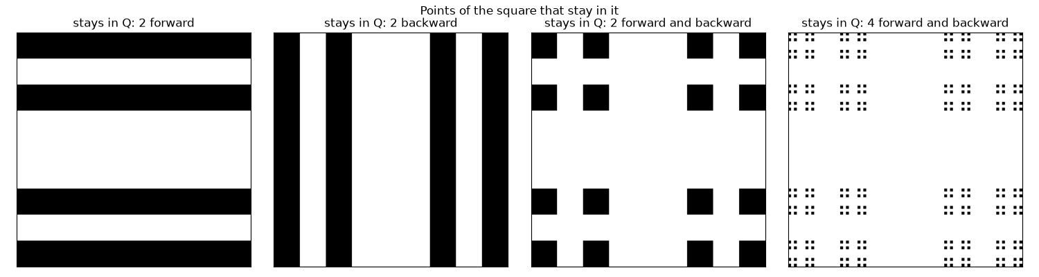
Points that stay in \(Q\) for \(n\) forward iterations fill \(2^n\) horizontal strips. Points that stay for \(n\) backward iterations fill \(2^n\) vertical strips. The points that do both fill \(4^n\) small squares, each of side \(3^{-n}\) here. survives() tests this for a grid of points. As \(n \to \infty\) the squares shrink to the invariant set \(\Lambda\), the product of two middle-thirds Cantor sets.

resolution = 729
centers = (np.arange(resolution) + 0.5) / resolution
grid = np.stack(np.meshgrid(centers, centers), axis=-1)

fig2, axes = plt.subplots(1, 4, figsize=(15, 4))
cases = [(2, 0, "2 forward"), (0, 2, "2 backward"), (2, 2, "2 forward and backward"), (4, 4, "4 forward and backward")]
for ax, (n_fwd, n_bwd, label) in zip(axes, cases):
    mask = system.survives(grid, n_forward=n_fwd, n_backward=n_bwd)
    ax.imshow(mask, origin="lower", extent=(0, 1, 0, 1), cmap="Greys", vmin=0, vmax=1)
    ax.set_title(f"stays in Q: {label}")
    ax.set_xticks([])
    ax.set_yticks([])
fig2.suptitle("Points of the square that stay in it")
fig2.tight_layout()

Symbolic dynamics: one orbit per symbol sequence

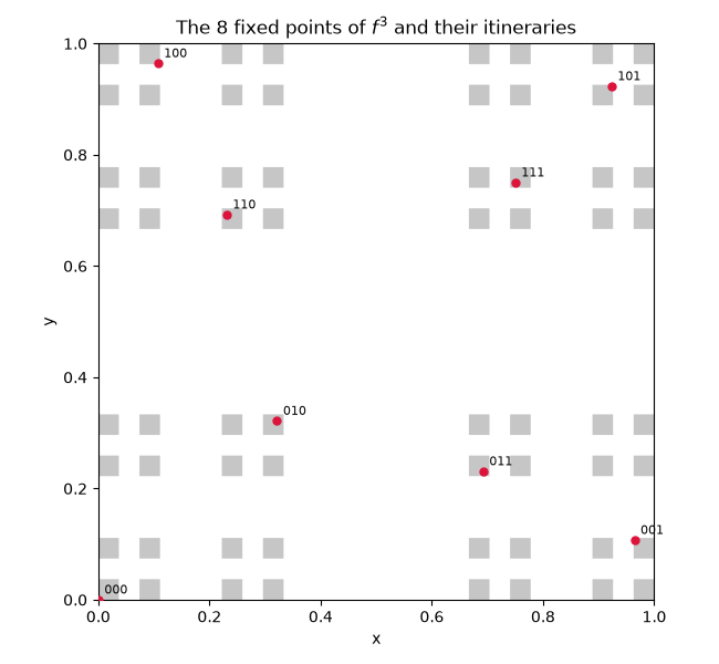
Record, for a point of \(\Lambda\), whether each iterate is in \(H_0\) or \(H_1\). Every bi-infinite sequence of 0s and 1s occurs, and it fixes the point uniquely. A periodic sequence gives a periodic orbit, so \(f^n\) has exactly \(2^n\) fixed points. Each branch acts affinely on \(x\) and \(y\) separately, so periodic_points() computes them all exactly. Below, the period-3 points are labeled by their itineraries and drawn on the squares that survive 3 iterations.

period = 3
points = system.periodic_points(period)
mask3 = system.survives(grid, n_forward=period, n_backward=period)

fig3, ax_p = plt.subplots(figsize=(6.5, 6))
ax_p.imshow(mask3, origin="lower", extent=(0, 1, 0, 1), cmap="Greys", vmin=0, vmax=3)
ax_p.scatter(points[:, 0], points[:, 1], color=theme.ACCENT, s=25, zorder=3)
for code, (px, py) in enumerate(points):
    ax_p.annotate(format(code, f"0{period}b"), (px, py), xytext=(4, 4), textcoords="offset points", fontsize=8)
ax_p.set_xlabel("x")
ax_p.set_ylabel("y")
ax_p.set_title(f"The {2**period} fixed points of $f^{period}$ and their itineraries")
fig3.tight_layout()

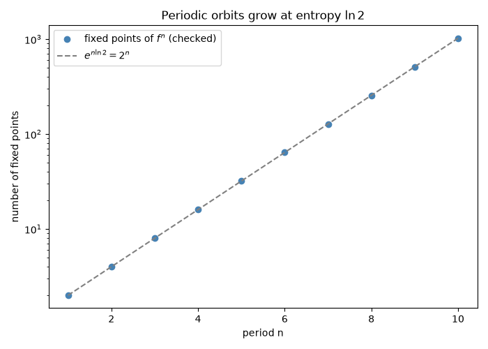
The count of periodic points grows as \(2^n\), so the topological entropy is \(\ln 2\). Iterating each computed point \(n\) times brings it back to itself, a check on the closed form.

periods = np.arange(1, 11)
counts = []
for n in periods:
    pts = system.periodic_points(n)
    images = pts.copy()
    for _ in range(n):
        images = system.fold(images)
    counts.append(np.sum(np.linalg.norm(images - pts, axis=1) < 1e-6))
counts = np.array(counts)

fig4, ax_n = plt.subplots(figsize=(7, 5))

ax_n.semilogy(periods, counts, "o", color=theme.PRIMARY, label="fixed points of $f^n$ (checked)")
ax_n.semilogy(periods, np.exp(system.topological_entropy() * periods), "--", color=theme.MUTED, label=r"$e^{n \ln 2} = 2^n$")
ax_n.set_xlabel("period n")
ax_n.set_ylabel("number of fixed points")
ax_n.set_title("Periodic orbits grow at entropy $\\ln 2$")
ax_n.legend()
fig4.tight_layout()

plt.show()

Check

f^n has exactly 2^n fixed points (one per binary itinerary), so the topological entropy is ln 2.

assert abs(system.topological_entropy() - np.log(2)) < 1e-12
np.testing.assert_array_equal(counts, 2**periods)
assert len(points) == 2**period