Standard Map

The Chirikov-Taylor standard map is an area-preserving (symplectic) map on the cylinder \((\theta, p) \in [0, 2\pi) \times [0, 2\pi)\), obtained by kicking a free rotor once per period with a torque \(k \sin\theta\):

\[p_{n+1} = p_n + k \sin\theta_n \pmod{2\pi}, \qquad \theta_{n+1} = \theta_n + p_{n+1} \pmod{2\pi}\]

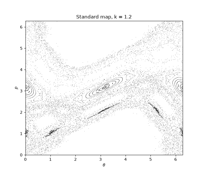
It is the textbook example of the transition from regularity to chaos: at low kick strength \(k\), most of phase space is filled with regular invariant curves (“islands”), i.e. \(k=0\) is integrable since every orbit then lies on a curve of constant \(p\); as \(k\) grows, these islands are progressively destroyed and replaced by a connected chaotic sea, with global chaos setting in around \(k \gtrsim 4\text{-}5\). This example reproduces the classic picture by iterating many initial conditions and overlaying their orbits.

import matplotlib.pyplot as plt
import numpy as np

from physicskit.chaos.systems.maps import StandardMap
from physicskit.chaos.utils.metrics import map_lyapunov_spectrum
from physicskit.chaos.visualizers.dynamic_plots import animate_multi_orbit_map

Sweep initial momenta

For a fixed kick strength, iterate a grid of initial conditions spanning the momentum axis to get one orbit per initial condition.

k = 1.2
system = StandardMap(k=k)
initial_momenta = np.linspace(0.05, np.pi - 0.05, 40)
orbits = [system.trajectory(np.array([0.0, p0]), n_iter=400) for p0 in initial_momenta]

Animation: the portrait filling in, iteration by iteration

All 40 orbits grow together, one new iterate per frame: watch some initial momenta trace out a closed, quasi-periodic loop around a regular island, while others scatter densely across the connected chaotic sea – a distinction that is easy to miss once every orbit is fully overlaid at once.

anim = animate_multi_orbit_map(
    orbits,
    xlim=(0.0, 2.0 * np.pi),
    ylim=(0.0, 2.0 * np.pi),
    labels=(r"$\theta$", "$p$"),
    title=f"Standard map, k = {k}",
)

plt.show()

To save the animation to a file instead of (or in addition to) displaying it interactively, use e.g.:

anim.save("standard_map_animation.gif", writer="pillow", fps=16)

The finished portrait

fig, ax = plt.subplots(figsize=(7, 6))
for traj in orbits:
    ax.plot(traj[:, 0], traj[:, 1], ",", color="black", alpha=0.6)

ax.set_xlim(0.0, 2.0 * np.pi)
ax.set_ylim(0.0, 2.0 * np.pi)
ax.set_xlabel(r"$\theta$")
ax.set_ylabel(r"$p$")
ax.set_title(f"Standard map, k = {k}")

plt.show()

Quantifying the transition: the largest Lyapunov exponent vs. k

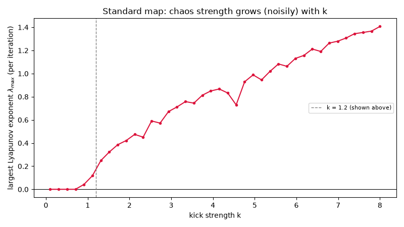
The portrait above only shows the mix of islands and chaotic sea at one kick strength. Sweeping k and estimating the largest Lyapunov exponent at each value with map_lyapunov_spectrum() (started from a generic initial condition, off any obvious island) turns “the sea grows as k increases” into a number: near-zero for the near-integrable small-k map, then trending positive and increasingly noisy (as the orbit samples islands of different sizes at different k) once global chaos sets in beyond k ~= 4-5.

k_values = np.linspace(0.1, 8.0, 40)
lambda_max = np.array([map_lyapunov_spectrum(StandardMap(k=float(k_i)), np.array([0.37, 1.83]), n_iter=4000, n_transient=500)[0] for k_i in k_values])

fig2, ax2 = plt.subplots(figsize=(8, 4.5))
ax2.axhline(0.0, color="black", lw=0.8)
ax2.plot(k_values, lambda_max, "o-", color="crimson", markersize=3)
ax2.axvline(k, color="gray", ls="--", lw=1.0, label=f"k = {k} (shown above)")
ax2.set_xlabel("kick strength k")
ax2.set_ylabel(r"largest Lyapunov exponent $\lambda_{max}$ (per iteration)")
ax2.set_title("Standard map: chaos strength grows (noisily) with k")
ax2.legend(fontsize=8)
fig2.tight_layout()

plt.show()