Cartwright–Littlewood: Chaos in the Forced Van der Pol Oscillator

In 1945 Mary Cartwright and J. E. Littlewood studied the valve oscillator equation of radar engineering, driven by a periodic signal,

\[\ddot{x} - \mu (1 - x^2) \dot{x} + x = A \cos(\omega t), \qquad A = b\, \omega \mu,\]

in the relaxation limit of large \(\mu\) (their \(k\); their \(\lambda\) is \(\omega\)). They proved that for a range of \(b\) it has two stable periodic motions with different periods at the same parameter values – subharmonics whose periods are different odd multiples of the forcing period \(T = 2\pi/\omega\) – together with a “bad” invariant set containing infinitely many periodic and uncountably many non-periodic orbits: chaos, proved in an equation from physics 18 years before Lorenz.

This example uses physicskit.chaos.systems.continuous.ForcedVanDerPol at \(\mu = 10\), \(\omega = 2.5\), \(b = 0.58\), where subharmonics of period \(3T\) and \(5T\) coexist, and shows the three pieces of their theorem in turn: (a) the two stable periodic motions, (b) the map of which starting points end up on which, and (c) the bad set sitting on the boundary between the two basins.

import matplotlib.pyplot as plt
import numpy as np
from matplotlib.colors import ListedColormap

from physicskit.chaos.systems.continuous import ForcedVanDerPol

mu, omega, b = 10.0, 2.5, 0.58
system = ForcedVanDerPol(mu=mu, A=b * omega * mu, omega=omega)
T = system.forcing_period
steps = 300  # RK4 steps per forcing period (basins are converged at this step)


def settled_period(samples, max_period=12, atol=1e-3):
    """Smallest p with x_{n+p} = x_n over the stroboscopic samples, else 0."""
    for p in range(1, max_period + 1):
        if np.allclose(samples[p:], samples[:-p], atol=atol):
            return p
    return 0

(a) Two stable periodic motions of different periods

Sampling the state once per forcing period (a stroboscopic map, via stroboscopic_map()) turns a periodic motion of period \(nT\) into an \(n\)-cycle of points. Two starting points only \(0.1\) apart in velocity settle, after the transient, onto different attractors: one relaxation cycle every \(3T\), or one every \(5T\).

starts = np.array([[0.5, -14.3], [0.5, -14.2]])
strobe = system.stroboscopic_map(starts, n_periods=150, steps_per_period=steps)
periods = [settled_period(s[-36:, 0]) for s in strobe]
print("settled periods (in units of T):", periods)

colors = {3: "tab:blue", 5: "tab:red"}
cycles = {}
fig, (ax_phase, ax_time) = plt.subplots(1, 2, figsize=(13, 5), gridspec_kw={"width_ratios": [1, 1.6]})
for s, p in zip(strobe, periods, strict=True):
    t, states = system.trajectory(state0=s[-1], dt=T / steps, n_steps=15 * steps)
    cycles[p] = s[-p:]
    ax_phase.plot(states[:, 0], states[:, 1], color=colors[p], lw=1.0, label=f"period {p}T")
    ax_phase.plot(s[-p:, 0], s[-p:, 1], "o", color=colors[p], ms=7, mec="k")
    ax_time.plot(t / T, states[:, 0], color=colors[p], lw=1.2, label=f"period {p}T")
    ax_time.plot(np.arange(16), states[::steps, 0], "o", color=colors[p], ms=5, mec="k")
ax_phase.set_xlabel("x")
ax_phase.set_ylabel(r"$\dot{x}$")
ax_phase.set_title("Phase portraits (dots: once per forcing period)")
ax_phase.legend(loc="upper left")
ax_time.set_xlabel("t / T  (forcing periods)")
ax_time.set_ylabel("x")
ax_time.set_title("Same parameters, two stable subharmonics: 3T and 5T")
ax_time.set_xticks(np.arange(0, 16))
ax_time.grid(axis="x", alpha=0.3)
fig.suptitle(rf"(a) Forced Van der Pol, $\mu={mu:g}$, $\omega={omega:g}$, $A=b\omega\mu$ with $b={b:g}$")
fig.tight_layout()

plt.show()

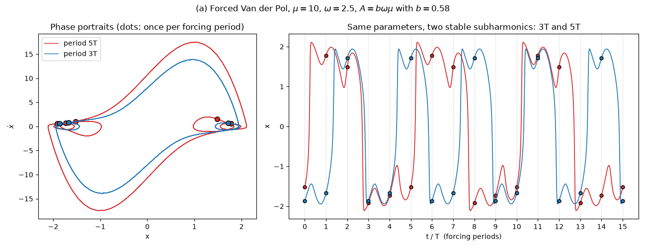
settled periods (in units of T): [5, 3]

(b) Which starting point ends up on which orbit?

Integrating a grid of starting points \((x_0, \dot{x}_0)\) at \(t = 0\) and colouring each by the period it settles onto maps the two basins of attraction. They interleave in ever-thinner bands. The boundary between them is where Cartwright and Littlewood’s bad set lives: a point exactly on it belongs to neither basin.

n_grid = 160
xs = np.linspace(-3.0, 3.0, n_grid)
vs = np.linspace(-1.5 * mu, 1.5 * mu, n_grid)
X, V = np.meshgrid(xs, vs)
grid = system.stroboscopic_map(np.column_stack([X.ravel(), V.ravel()]), n_periods=100, steps_per_period=steps)
labels = np.array([settled_period(s[-36:, 0]) for s in grid]).reshape(n_grid, n_grid)
print("grid points settling on each period:", {int(p): int(n) for p, n in zip(*np.unique(labels, return_counts=True), strict=True)})

fig2, ax2 = plt.subplots(figsize=(8, 7))
ax2.imshow(
    np.where(labels == 3, 0, 1),
    origin="lower",
    extent=(xs[0], xs[-1], vs[0], vs[-1]),
    aspect="auto",
    cmap=ListedColormap(["#9ecae1", "#fcaeae"]),
    interpolation="nearest",
)
for p, pts in cycles.items():
    ax2.plot(pts[:, 0], pts[:, 1], "o", color=colors[p], ms=9, mec="k", label=f"stable {p}T cycle")
ax2.set_xlabel(r"$x_0$")
ax2.set_ylabel(r"$\dot{x}_0$")
ax2.set_title("(b) Basins: blue settles on the 3T orbit, red on the 5T orbit")
ax2.legend(loc="upper right")
fig2.tight_layout()

plt.show()

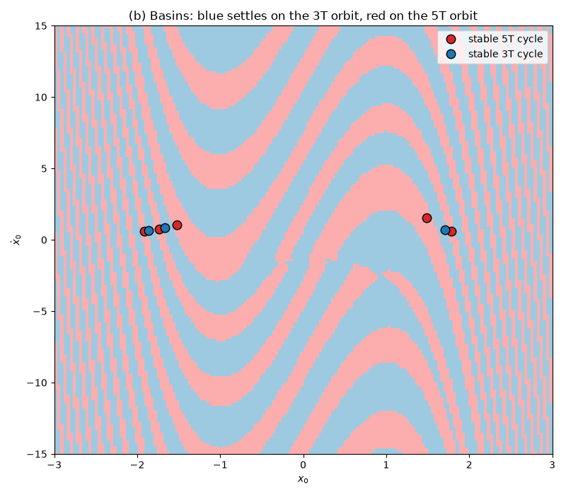
grid points settling on each period: {3: 14343, 5: 11257}

(c) The bad set: an orbit that wanders irregularly, then settles

The bad set is repelling: nearby orbits leave it at a rate of roughly \(e^{2.8}\) per forcing period, so a single double-precision trajectory aimed at the boundary stays near it for only about a dozen periods. The straddle method (Nusse and Yorke, 1989) keeps it there for as long as we like. We keep a pair of points on opposite sides of the boundary, advance both by one period, and bisect between them again whenever they drift apart. Their midpoint then follows an orbit on the bad set. After 60 forcing periods we stop correcting it and let it go.

def fates(points):
    s = system.stroboscopic_map(points, n_periods=100, steps_per_period=steps)
    return np.array([settled_period(q[-36:, 0]) for q in s])


def refine(a, c, fate_a, tol=1e-9):
    """Shrink the straddling pair (a, c) to within tol, keeping fates apart."""
    scale = np.array([1.0, 1.0 / mu])
    while np.linalg.norm((c - a) * scale) > tol:
        pts = a + np.linspace(0.0, 1.0, 11)[1:-1, None] * (c - a)
        other = np.flatnonzero(fates(pts) != fate_a)
        if other.size == 0:
            a = pts[-1]
            continue
        j = other[0]
        a, c = (pts[j - 1] if j > 0 else a), pts[j]
    return a, c


a, c = starts[0].copy(), starts[1].copy()
fate_a = periods[0]
n_track, n_free = 60, 30
tracked = []
for _ in range(n_track):
    a, c = refine(a, c, fate_a)
    tracked.append(0.5 * (a + c))
    a, c = system.stroboscopic_map(np.array([a, c]), n_periods=1, steps_per_period=steps)[:, -1]
released = system.stroboscopic_map(tracked[-1], n_periods=n_free, steps_per_period=steps)[0, 1:]
samples = np.vstack([tracked, released])

# Continuous x(t): each tracked point is integrated for one period (the
# pieces join to within 1e-9), then the released orbit runs on freely.
pieces = [system.trajectory(state0=p, dt=T / steps, n_steps=steps)[1][:-1] for p in tracked]
pieces.append(system.trajectory(state0=tracked[-1], dt=T / steps, n_steps=(n_free + 1) * steps)[1][steps:])
x_path = np.concatenate(pieces)[:, 0]
t_path = np.arange(x_path.size) * (T / steps) / T


def cycle_lengths(x, t, level=1.0):
    """Time between successive upward relaxation jumps, in forcing periods.

    A jump is an upward crossing of x = +1: the lower-branch wiggles and the
    aborted jumps of the bad set, which hover near x = 0, never reach it.
    """
    up = np.flatnonzero((x[:-1] < level) & (x[1:] >= level))
    t_up = t[up] + (level - x[up]) * (t[up + 1] - t[up]) / (x[up + 1] - x[up])
    return t_up[1:], np.diff(t_up)


t_cyc, lengths = cycle_lengths(x_path, t_path)
final_period = settled_period(released[-15:, 0])
print(f"bad-set cycle lengths (in T): {np.round(lengths[t_cyc < n_track], 2).tolist()}")
print(f"released orbit settles on period {final_period}T")

fig3, (ax_x, ax_len) = plt.subplots(2, 1, figsize=(13, 7), sharex=True)
ax_x.axvspan(0, n_track, color="0.92", zorder=0, label="kept on the bad set")
ax_x.plot(t_path, x_path, color="k", lw=0.9)
ax_x.plot(np.arange(samples.shape[0]), samples[:, 0], "o", color="tab:purple", ms=3.5)
ax_x.set_ylabel("x")
ax_x.set_title(f"(c) An orbit on the bad set wanders irregularly for {n_track} periods, then settles onto the {final_period}T orbit")
ax_x.legend(loc="upper right")

ax_len.step(t_cyc, lengths, where="pre", color="tab:purple", lw=1.5, label="this orbit")
for p in (3, 5):
    ax_len.axhline(p, color=colors[p], ls="--", lw=1.2, label=f"stable {p}T orbit")
ax_len.axvline(n_track, color="0.4", lw=1.0)
ax_len.set_xlabel("t / T  (forcing periods)")
ax_len.set_ylabel("period of each\nrelaxation cycle (T)")
ax_len.set_ylim(1.5, 6.5)
ax_len.legend(loc="upper left", ncol=3)
fig3.tight_layout()

plt.show()

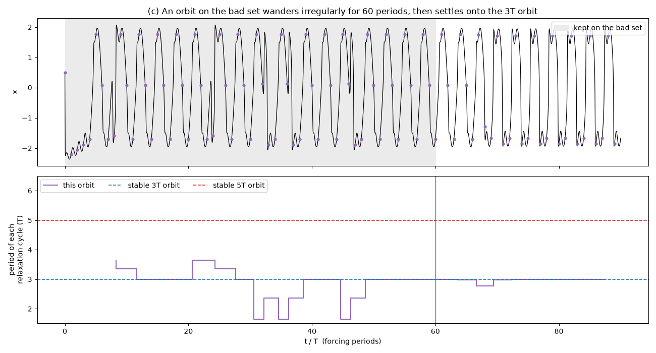
bad-set cycle lengths (in T): [3.64, 3.36, 3.0, 3.0, 3.0, 3.64, 3.36, 3.0, 1.64, 2.36, 1.64, 2.36, 3.0, 3.0, 1.64, 2.36, 3.0, 3.0, 3.0]
released orbit settles on period 3T

The stable orbits repeat one fixed cycle length, 3 or 5 forcing periods. The bad-set orbit keeps hovering near the unstable middle branch \(x \approx 0\) (the purple samples there), sometimes falling back and sometimes jumping late. So its cycles have irregular, non-integer lengths in a non-repeating order. Cartwright and Littlewood proved that the bad set holds infinitely many periodic and uncountably many non-periodic orbits. Levinson’s 1949 piecewise-linear model showed the same structure more explicitly, and it was that example that led Smale to the horseshoe.

Check

Cartwright and Littlewood: at the same parameters two stable subharmonics (3T and 5T) coexist, each with a large basin, and the boundary between them carries orbits whose relaxation cycles have irregular lengths (the ‘bad set’) before settling.

assert sorted(periods) == [3, 5]
values, counts = np.unique(labels, return_counts=True)
assert set(values.tolist()) == {3, 5} and counts.min() > 0.2 * labels.size
bad = lengths[t_cyc < n_track]
assert np.any(np.abs(bad - 3) > 0.2) and np.any(np.abs(bad - 5) > 0.2) and final_period in (3, 5)