Chua’s Circuit: the Double-Scroll Attractor

Chua’s circuit is built from just a handful of standard electronic components – two capacitors, one inductor, one resistor, and a single piecewise-linear nonlinear resistor (the “Chua diode”) – yet it is chaotic. In dimensionless variables \((x, y, z)\) (proportional to the two capacitor voltages and the inductor current), its dynamics are

\[\begin{split}\dot{x} &= \alpha (y - x - h(x)) \\ \dot{y} &= x - y + z \\ \dot{z} &= -\beta y \\ h(x) &= m_1 x + \tfrac{1}{2}(m_0 - m_1)\left(|x + 1| - |x - 1|\right)\end{split}\]

where \(h(x)\) is the Chua diode’s piecewise-linear current-voltage characteristic (slope \(m_0\) near the origin, \(m_1\) for large \(|x|\)), and \(\alpha\), \(\beta\) are ratios of the circuit’s capacitances and inductance. It holds a special place in chaos theory as the first system whose chaotic behavior was confirmed both by simulation and by direct physical experiment in real hardware, closing the “is chaos just a numerical artifact?” question of the 1980s. For the classic parameters (\(\alpha=15.6\), \(\beta=28\), \(m_0=-8/7\), \(m_1=-5/7\)) it produces the famous double-scroll attractor. Alongside the attractor itself, physicskit.chaos.visualizers.divergence.plot_lyapunov_divergence() quantifies the “chaotic” claim directly, by tracking how fast two initially nearby trajectories separate.

import matplotlib.pyplot as plt

from physicskit.chaos.systems.continuous import Chua
from physicskit.chaos.visualizers.divergence import plot_lyapunov_divergence

system = Chua(alpha=15.6, beta=28.0)

Integrate

t, states = system.trajectory(n_steps=40000, dt=0.01)
states = states[2000:]

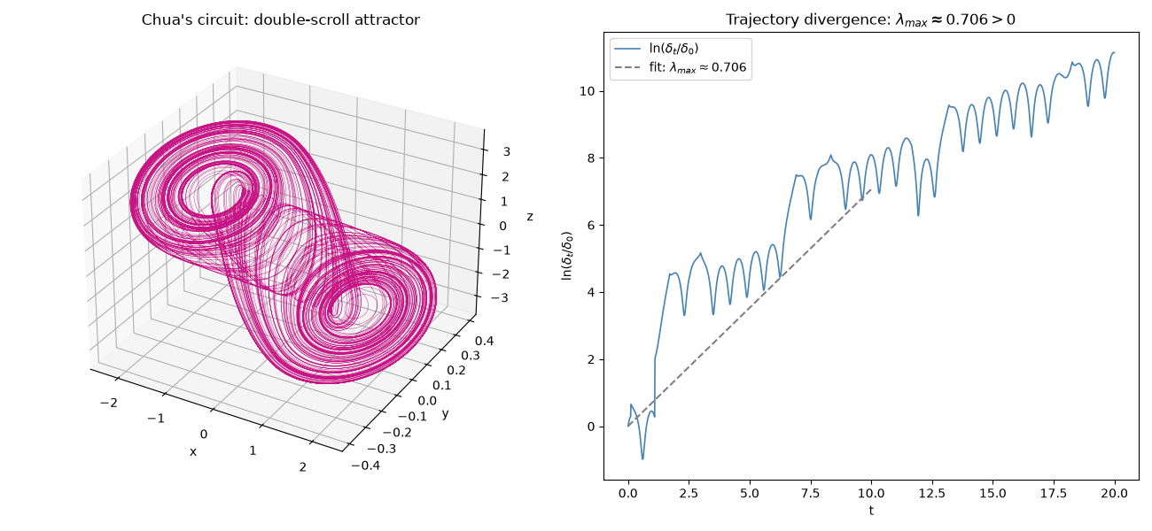
The double scroll, and the divergence that makes it chaotic

The trajectory spirals outward on one lobe, crosses over, spirals outward on the other, and back again – unpredictably, forever. Alongside it, plot_lyapunov_divergence() makes the “chaotic” claim quantitative: two trajectories launched an infinitesimal distance apart separate exponentially, at a rate \(\lambda_{\max} > 0\).

fig = plt.figure(figsize=(13, 6))
ax = fig.add_subplot(1, 2, 1, projection="3d")
ax.plot(states[:, 0], states[:, 1], states[:, 2], lw=0.3, color="mediumvioletred")
ax.set_xlabel("x")
ax.set_ylabel("y")
ax.set_zlabel("z")
ax.set_title("Chua's circuit: double-scroll attractor")

ax_div = fig.add_subplot(1, 2, 2)
_, _, lam = plot_lyapunov_divergence(system, t_max=20.0, n_points=1500, ax=ax_div, seed=0)
ax_div.set_title(f"Trajectory divergence: $\\lambda_{{max}} \\approx {lam:.3f} > 0$")
fig.tight_layout()

plt.show()