Double Pendulum

The double pendulum is a simple mechanical system – two point masses \(m_1\), \(m_2\) on massless rigid rods of length \(l_1\), \(l_2\), hanging from a fixed pivot under gravity \(g\), with no friction – whose motion is nonetheless chaotic for large enough swings. In terms of the two rod angles \(\theta_1, \theta_2\) from vertical and their angular velocities \(\omega_1 = \dot\theta_1\), \(\omega_2 = \dot\theta_2\), the equations of motion are

\[\begin{split}\dot\omega_1 &= \frac{-g(2m_1+m_2)\sin\theta_1 - m_2 g \sin(\theta_1 - 2\theta_2) - 2\sin(\theta_1-\theta_2)\, m_2 \left(\omega_2^2 l_2 + \omega_1^2 l_1 \cos(\theta_1-\theta_2)\right)} {l_1 \left(2m_1 + m_2 - m_2 \cos(2\theta_1 - 2\theta_2)\right)} \\ \dot\omega_2 &= \frac{2 \sin(\theta_1-\theta_2)\left(\omega_1^2 l_1 (m_1+m_2) + g(m_1+m_2)\cos\theta_1 + \omega_2^2 l_2 m_2 \cos(\theta_1-\theta_2)\right)} {l_2 \left(2m_1 + m_2 - m_2 \cos(2\theta_1 - 2\theta_2)\right)}\end{split}\]

with \(\dot\theta_1=\omega_1\), \(\dot\theta_2=\omega_2\). This example integrates a trajectory with physicskit.chaos.systems.continuous.DoublePendulum.trajectory(), traces the path of the outer bob, and checks how well the integrator conserves total mechanical energy using physicskit.chaos.utils.metrics.energy_drift().

import matplotlib.pyplot as plt
import numpy as np

from physicskit.chaos.systems.continuous import DoublePendulum
from physicskit.chaos.utils.metrics import energy_drift
from physicskit.chaos.visualizers.dynamic_plots import animate_double_pendulum

system = DoublePendulum(m1=1.0, m2=1.0, l1=1.0, l2=1.0, g=9.81)
state0 = np.array([np.pi / 2, np.pi / 2, 0.0, 0.0])

Animation: the pendulum swinging, arms and all

Rendered kinematically – the two rigid rods and bobs swinging in real space – rather than only as an abstract (theta, omega) trajectory.

anim = animate_double_pendulum(system, state0=state0, dt=0.005, n_steps=10000, skip=20)

plt.show()

To save the animation to a file instead of (or in addition to) displaying it interactively, use e.g.:

anim.save("double_pendulum_animation.gif", writer="pillow", fps=30)

Integrate

Start from a near-horizontal, at-rest configuration – energetic enough to be chaotic.

t, states = system.trajectory(state0=state0, n_steps=8000, dt=0.005)

Outer bob trajectory

Convert the generalized coordinates (theta1, theta2) to the Cartesian position of the second (outer) bob.

th1, th2 = states[:, 0], states[:, 1]
x2 = system.l1 * np.sin(th1) + system.l2 * np.sin(th2)
y2 = -system.l1 * np.cos(th1) - system.l2 * np.cos(th2)

fig, ax = plt.subplots(figsize=(6, 6))
ax.plot(x2, y2, lw=0.4, color="indigo")
ax.set_aspect("equal")
ax.set_title("Double pendulum: outer bob trajectory")

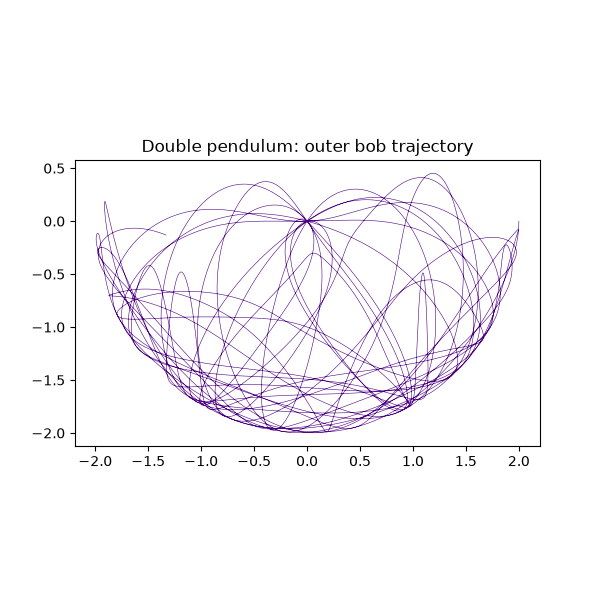
Text(0.5, 1.0, 'Double pendulum: outer bob trajectory')

Energy conservation check

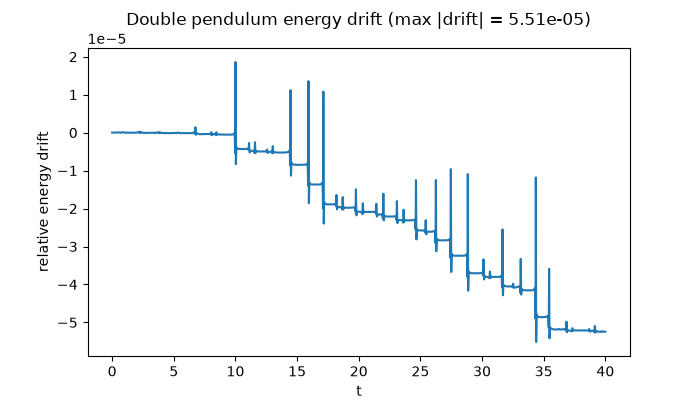
The double pendulum is a conservative system, so total mechanical energy should stay (nearly) constant; the small residual drift below reflects the RK4 integrator’s local truncation error rather than any physical damping.

drift = energy_drift(t, states, system.energy)

fig2, ax2 = plt.subplots(figsize=(7, 4))
ax2.plot(t, drift)
ax2.set_xlabel("t")
ax2.set_ylabel("relative energy drift")
ax2.set_title(f"Double pendulum energy drift (max |drift| = {np.max(np.abs(drift)):.2e})")

plt.show()