Driven Pendulum: the Period-Doubling Route to Chaos

The sinusoidally forced, damped pendulum obeys

\[\ddot\theta + \gamma \dot\theta + \frac{g}{l}\sin\theta = A \cos(\omega_d t),\]

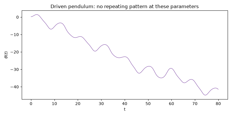
or, as the first-order system in \((\theta, \omega)\) actually integrated, \(\dot\theta = \omega\), \(\dot\omega = -\gamma\omega - (g/l)\sin\theta + A\cos(\omega_d t)\), where \(\gamma\) is the viscous damping coefficient, \(g/l\) is the small-angle frequency squared of the undamped, undriven pendulum, and \(A\), \(\omega_d\) are the forcing torque’s amplitude and angular frequency. It is the classic mechanical system for the period-doubling route to chaos: D’Humieres, Beasley, Huberman, and Libchaber (1982) showed experimentally that sweeping the forcing amplitude \(A\) reproduces the same cascade of period-doubling bifurcations as the logistic map, this time in a genuine forced mechanical oscillator. At the default (deep-chaotic) parameters below, the pendulum’s swing never settles into a repeating pattern.

import matplotlib.pyplot as plt
import numpy as np

from physicskit.chaos.systems.continuous import DrivenPendulum
from physicskit.chaos.visualizers.bifurcation import plot_bifurcation_diagram, stroboscopic_bifurcation_sampler

system = DrivenPendulum(damping=0.5, g_over_l=1.0, A=1.5, omega_d=2.0 / 3.0)

A single trajectory

t, states = system.trajectory(n_steps=4000, dt=0.02)
theta = states[:, 0]

fig, ax = plt.subplots(figsize=(8, 4))
ax.plot(t, theta, lw=0.6, color="indigo")
ax.set_xlabel("t")
ax.set_ylabel(r"$\theta(t)$")
ax.set_title("Driven pendulum: no repeating pattern at these parameters")
fig.tight_layout()

The period-doubling route to chaos

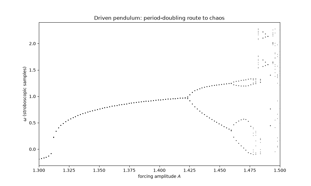
Sampling the angular velocity omega once per forcing period turns the continuous flow into an effective discrete map – the same stroboscopic-sampling trick used for the Duffing oscillator (omega, unlike theta, stays bounded even while the pendulum occasionally rotates over the top). Sweeping the forcing amplitude A over this narrow window reveals the same period-doubling cascade Feigenbaum found in the abstract logistic map – period-1, then period-2, period-4, and a chaotic band, interrupted by a periodic window – now in a physically forced pendulum.

period = 2.0 * np.pi / system.omega_d

sampler = stroboscopic_bifurcation_sampler(
    lambda A: DrivenPendulum(damping=0.5, g_over_l=1.0, A=A, omega_d=2.0 / 3.0),
    state0=np.array([0.2, 0.0]),
    sample_period=period,
    n_transient_periods=60,
    n_keep_periods=16,
    component=1,
    dt=0.1,
    rtol=1e-6,
    atol=1e-8,
)

A_values = np.linspace(1.30, 1.50, 100)
fig2, ax2 = plot_bifurcation_diagram(A_values, sampler, n_jobs=4, marker=".", markersize=1.0)
ax2.set_xlabel(r"forcing amplitude $A$")
ax2.set_ylabel(r"$\omega$ (stroboscopic samples)")
ax2.set_title("Driven pendulum: period-doubling route to chaos")

plt.show()