Duffing Oscillator

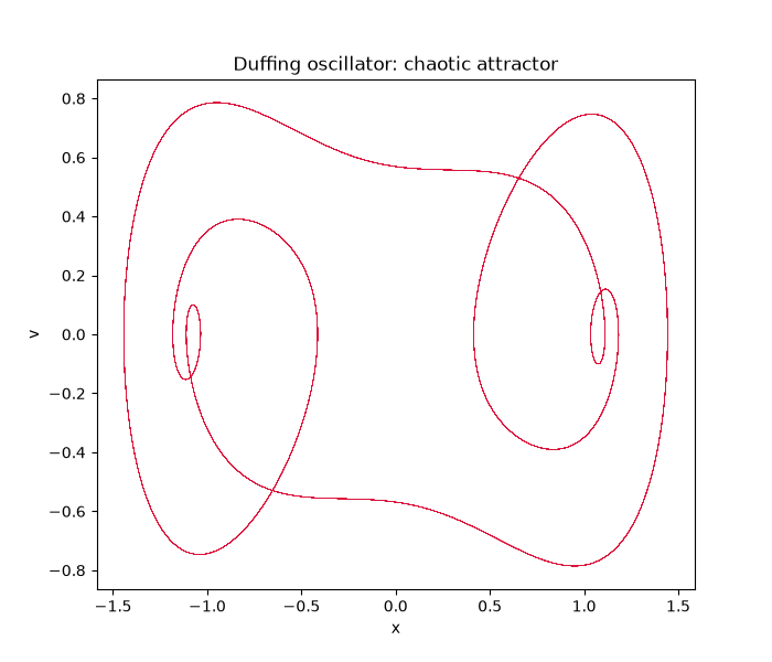
The forced, damped Duffing oscillator models a particle in a double-well potential driven by a periodic force,

\[\ddot{x} + \delta \dot{x} + \alpha x + \beta x^3 = \gamma \cos(\omega t),\]

or, as the first-order system in \((x, v)\) actually integrated, \(\dot{x} = v\), \(\dot{v} = -\delta v - \alpha x - \beta x^3 + \gamma \cos(\omega t)\). Here \(\delta\) is the damping coefficient, \(\alpha\) and \(\beta\) set the (linear and cubic) restoring force – with \(\alpha<0\) and \(\beta>0\), as used below, the potential \(V(x)=\tfrac12\alpha x^2+\tfrac14\beta x^4\) has two wells – and \(\gamma\), \(\omega\) are the forcing amplitude and frequency. For the classic chaotic parameter set below, its long-time trajectory settles onto a strange attractor in the (x, v) phase plane.

import matplotlib.pyplot as plt

from physicskit.chaos.systems.continuous import Duffing
from physicskit.chaos.utils.dimension import box_counting_dimension, correlation_dimension

system = Duffing(delta=0.3, alpha=-1.0, beta=1.0, gamma=0.37, omega=1.2)

Integrate

Discard an initial transient so the plotted trajectory has already settled onto the attractor.

t, states = system.trajectory(n_steps=40000, dt=0.02)
states = states[5000:]

Phase portrait

fig, ax = plt.subplots(figsize=(7, 6))
ax.plot(states[:, 0], states[:, 1], lw=0.2, color="crimson")
ax.set_xlabel("x")
ax.set_ylabel("v")
ax.set_title("Duffing oscillator: chaotic attractor")

plt.show()

Quantifying it: a fractal attractor

The dense-but-structured phase portrait above is a strange attractor: its box-counting (capacity) dimension \(D_0\) and correlation dimension \(D_2\) (see Fractal Dimension: Box-Counting and Correlation Dimension for both estimators applied to the Henon map) are non-integers, between the curve (\(D=1\)) a single trajectory traces out locally and the 2D plane it never quite fills. Only every 4th stroboscopic-ish sample is kept for the correlation-dimension estimate, since it computes all \(O(n^2)\) pairwise distances.

d0, eps0, counts0 = box_counting_dimension(states)
d2, eps2, csum2 = correlation_dimension(states[::4])
print(f"Duffing attractor: box-counting D0 = {d0:.3f}, correlation D2 = {d2:.3f}")

fig2, axes2 = plt.subplots(1, 2, figsize=(12, 5))
axes2[0].loglog(1.0 / eps0, counts0, "o-", color="steelblue")
axes2[0].set_xlabel(r"$1/\epsilon$")
axes2[0].set_ylabel(r"$N(\epsilon)$")
axes2[0].set_title(f"Box counting: D0 = {d0:.3f}")

axes2[1].loglog(eps2, csum2, "o-", color="darkorange")
axes2[1].set_xlabel(r"$\epsilon$")
axes2[1].set_ylabel(r"$C(\epsilon)$")
axes2[1].set_title(f"Correlation sum: D2 = {d2:.3f}")
fig2.suptitle("Duffing attractor: fractal dimension between 1 (curve) and 2 (plane)")
fig2.tight_layout()

plt.show()

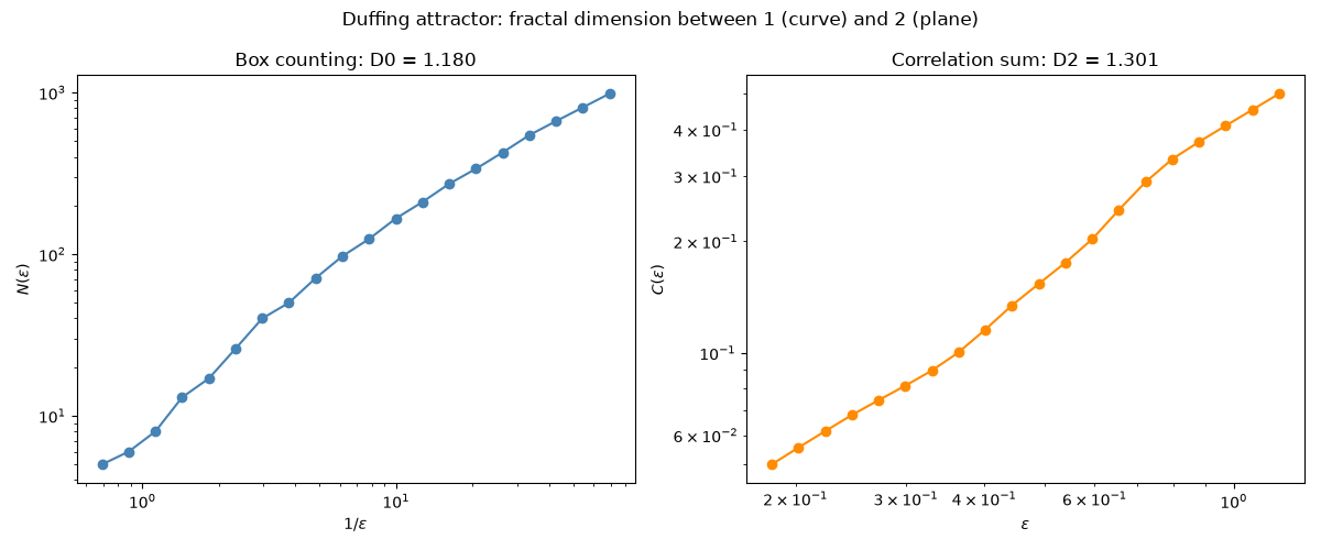
Duffing attractor: box-counting D0 = 1.180, correlation D2 = 1.301