Lorenz Attractor

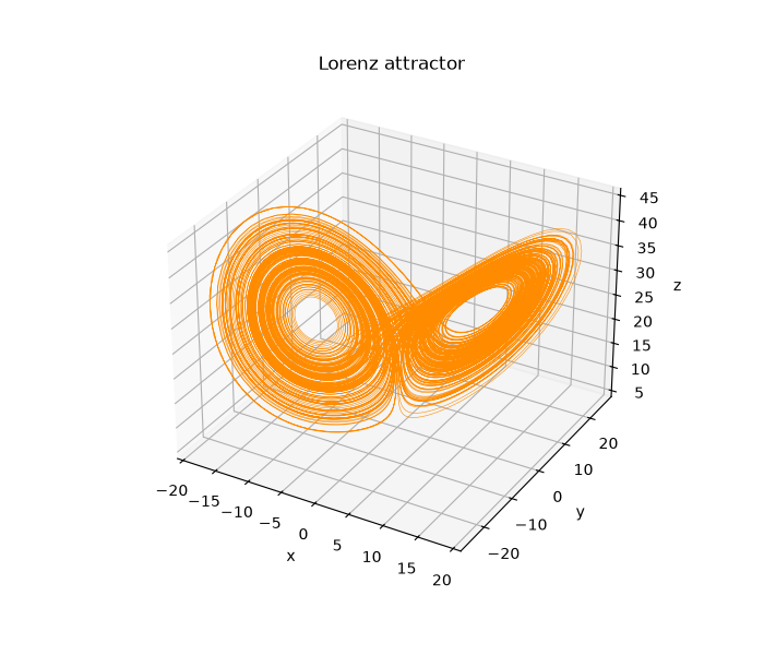
The Lorenz system is the archetypal chaotic flow: three coupled nonlinear autonomous ODEs, originally derived as a drastic truncation of the equations for atmospheric (Rayleigh-Benard) convection,

\[\begin{split}\dot{x} &= \sigma (y - x) \\ \dot{y} &= x (\rho - z) - y \\ \dot{z} &= x y - \beta z\end{split}\]

whose trajectories, for the classic parameters \(\sigma=10\), \(\rho=28\), \(\beta=8/3\) used below, settle onto a butterfly-shaped strange attractor rather than a fixed point or limit cycle. This example integrates a trajectory with physicskit.chaos.systems.continuous.Lorenz.trajectory() (the Numba-accelerated RK4 integrator) and plots it in 3D.

import matplotlib.pyplot as plt

from physicskit.chaos.systems.continuous import Lorenz
from physicskit.chaos.visualizers.section import plot_poincare_map

system = Lorenz(sigma=10.0, rho=28.0, beta=8.0 / 3.0)

Integrate

We discard a short initial transient so the plotted trajectory starts already on the attractor.

t, states = system.trajectory(n_steps=20000, dt=0.01)
states = states[500:]

Plot

fig = plt.figure(figsize=(7, 6))
ax = fig.add_subplot(projection="3d")
ax.plot(states[:, 0], states[:, 1], states[:, 2], lw=0.4, color="darkorange")
ax.set_xlabel("x")
ax.set_ylabel("y")
ax.set_zlabel("z")
ax.set_title("Lorenz attractor")

plt.show()

Poincare section: slicing the butterfly

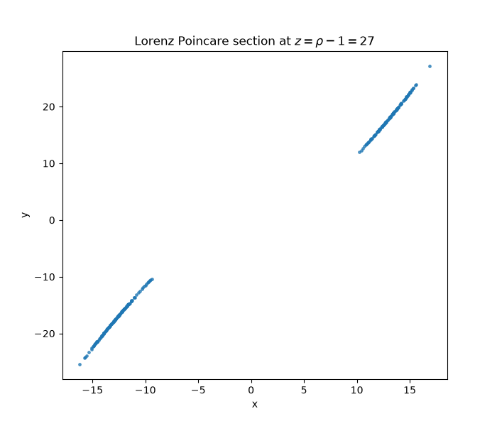
The tangled 3D curve above is far easier to read one slice at a time. plot_poincare_map() samples the flow only at the instants it pierces the plane \(z = \rho - 1 = 27\) (through the two unstable fixed points the attractor’s two lobes wind around) while ascending (\(\dot{z} > 0\)), and scatters each crossing’s \((x, y)\). Rather than a tangled ribbon, the result is two crisp, curved bands – one per lobe – whose thickness reveals the attractor’s fine, sheet-like layered structure directly, without the 3D projection’s self-occlusion.

fig2, ax2 = plot_poincare_map(
    system,
    system.initial_state(),
    coord=2,
    value=system.rho - 1.0,
    direction=1.0,
    plot_coords=(0, 1),
    t_max=200.0,
    dt=0.005,
)
ax2.set_xlabel("x")
ax2.set_ylabel("y")
ax2.set_title(rf"Lorenz Poincare section at $z = \rho - 1 = {system.rho - 1.0:g}$")

plt.show()