Quantum Billiard Eigenstates

A quantum particle confined to a 2D billiard – “particle in a box” with a chaotic (or not) box shape – is the other classic playground of quantum chaos, alongside quantized maps like the quantum kicked rotor. In units where \(\hbar^2/2m=1\), its stationary states solve the Dirichlet Helmholtz eigenproblem

\[-\nabla^2 \psi = k^2 \psi \quad \text{inside the billiard}, \qquad \psi = 0 \quad \text{on the boundary},\]

with energy eigenvalues \(E_n = k_n^2\). QuantumBilliard solves for these eigenstates for any billiard shape physicskit.chaos ships, using a simple five-point finite-difference discretization of the Laplacian – no shape-specific code needed.

import matplotlib.pyplot as plt

from physicskit.chaos.quantum import QuantumBilliard
from physicskit.chaos.systems.billiards import BunimovichStadium, CircleBilliard
from physicskit.chaos.visualizers import plot_billiard_eigenstate, plot_weyl_law

The integrable case: a circular billiard

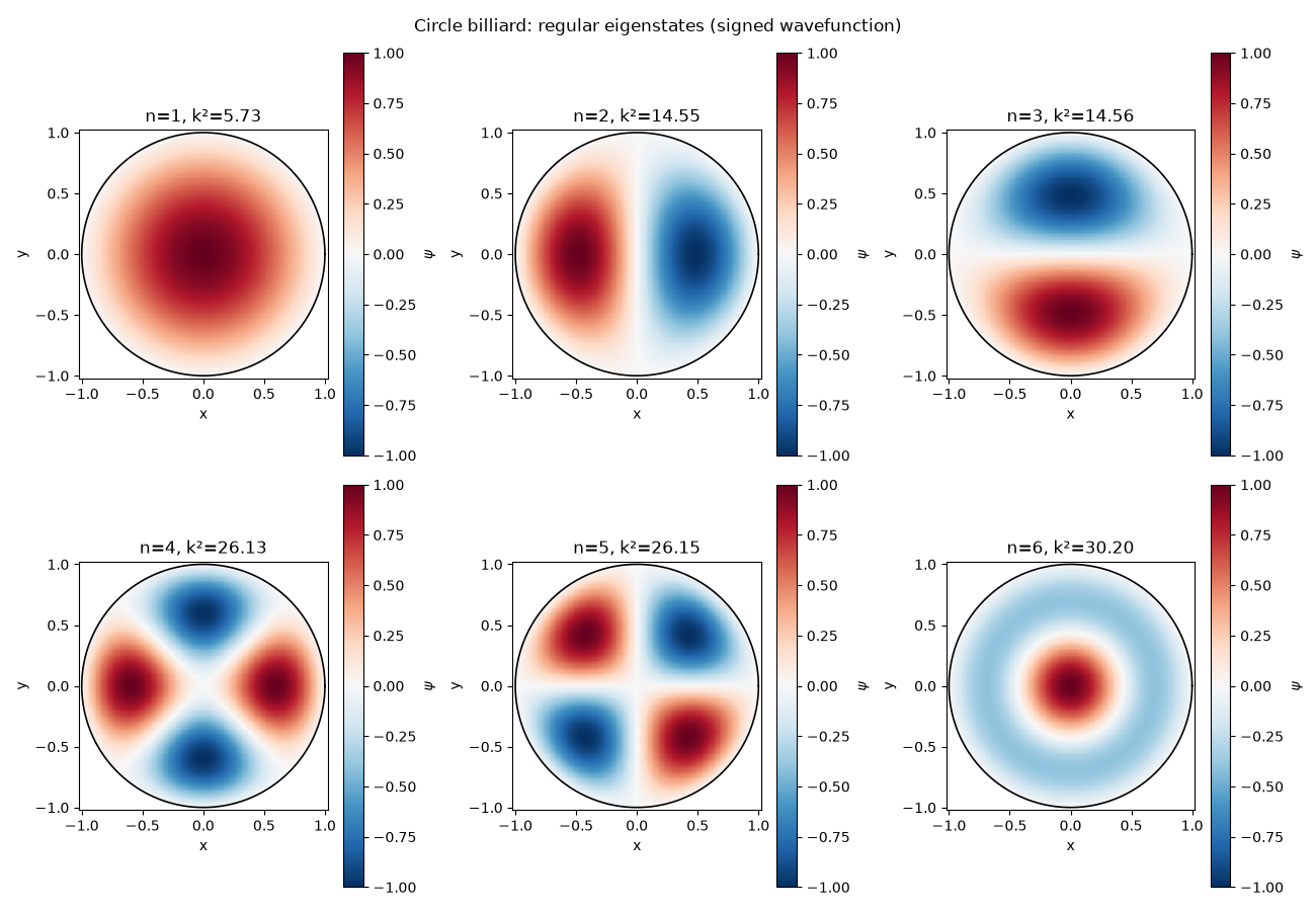
The circle is integrable, so its eigenstates come in near-degenerate pairs (except a few of the lowest) reflecting angular momentum, and each one’s nodal lines form a simple, regular grid of radial and angular lines.

circle = QuantumBilliard(CircleBilliard(radius=1.0), resolution=140)
eigenvalues, eigenfunctions = circle.eigenstates(n_states=6)

fig, axes = plt.subplots(2, 3, figsize=(13, 9))
for i, ax in enumerate(axes.flat):
    plot_billiard_eigenstate(circle, eigenfunctions[i], ax=ax, density=False)
    ax.set_title(f"n={i + 1}, k²={eigenvalues[i]:.2f}")
fig.suptitle("Circle billiard: regular eigenstates (signed wavefunction)")
fig.tight_layout()

plt.show()

The chaotic case: a Bunimovich stadium

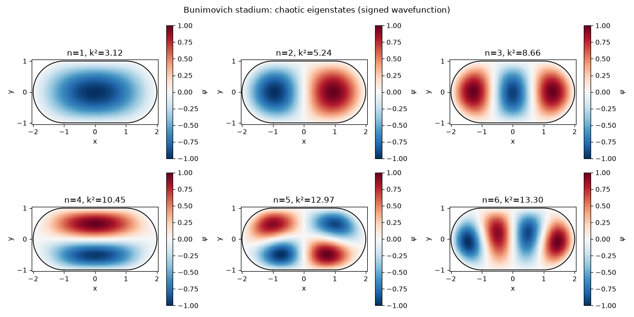
The stadium is a textbook chaotic billiard (see Bunimovich Stadium (Chaotic)): its eigenstates have no simple regular nodal pattern, and some show “scarring” – amplitude anomalously enhanced along an unstable classical periodic orbit, most famously the straight bouncing-ball path along the stadium’s long axis. Plotted the same way as the circle above (signed wavefunction, not just probability density) so the two are directly comparable: the finite- difference solver’s eigenvectors are real-valued either way, so a signed plot is always available and shows strictly more – both the nodal lines and the amplitude pattern – than density alone would.

stadium = QuantumBilliard(BunimovichStadium(radius=1.0, straight_length=2.0), resolution=140)
eigenvalues_s, eigenfunctions_s = stadium.eigenstates(n_states=6)

fig2, axes2 = plt.subplots(2, 3, figsize=(13, 6.5))
for i, ax in enumerate(axes2.flat):
    plot_billiard_eigenstate(stadium, eigenfunctions_s[i], ax=ax, density=False)
    ax.set_title(f"n={i + 1}, k²={eigenvalues_s[i]:.2f}")
fig2.suptitle("Bunimovich stadium: chaotic eigenstates (signed wavefunction)")
fig2.tight_layout()

plt.show()

Weyl’s law

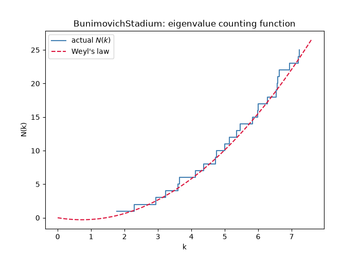
However irregular the individual eigenvalues, their counting function N(k) (the number of eigenvalues below k) always tracks Weyl’s law on average – a purely geometric prediction from the billiard’s area and perimeter alone, with no reference to whether the classical dynamics is regular or chaotic. This is a good sanity check on the eigensolver itself, independent of any known analytic spectrum.

fig3, ax3 = plot_weyl_law(stadium, n_states=25)

plt.show()