Quantum Kicked Rotor

The quantum kicked rotor is the quantization of physicskit.chaos’s classical StandardMap, \(p_{n+1} = p_n + k\sin\theta_n \pmod{2\pi}\), \(\theta_{n+1} = \theta_n + p_{n+1} \pmod{2\pi}\): a particle on a ring, kicked periodically by a potential \(k\cos\theta\). Its one-period evolution is the unitary Floquet operator

\[U = \mathcal{F}^{-1} \exp\!\left(-i\hbar \frac{m^2}{2}\right) \mathcal{F} \, \exp\!\left(-i \frac{k}{\hbar} \cos\theta\right),\]

alternating a kick phase \(\exp(-i (k/\hbar) \cos\theta)\) (diagonal in the angle representation) with a free-rotation (“kinetic”) phase \(\exp(-i\hbar m^2/2)\) (diagonal in the momentum representation, \(m\) the angular-momentum quantum number), connected by the discrete Fourier transform \(\mathcal{F}\). It is one of the two textbook models of quantum chaos (the other being a particle confined to a chaotic billiard – see Quantum Billiard Eigenstates), and the system in which dynamical localization – the quantum suppression of classical chaotic diffusion – was first understood.

import matplotlib.pyplot as plt
import numpy as np

from physicskit.chaos.quantum import QuantumKickedRotor
from physicskit.chaos.systems.maps import StandardMap
from physicskit.chaos.visualizers import animate_husimi_evolution, plot_husimi, plot_quantum_spectrum, theme

The Floquet spectrum

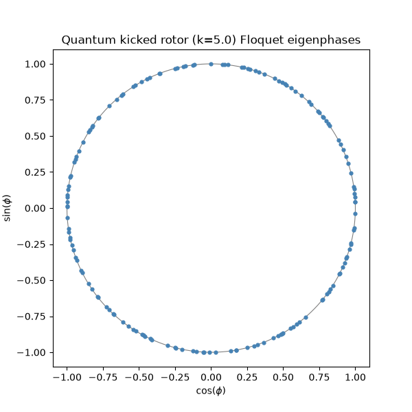
One period of kick-then-rotation is a unitary “Floquet” operator; its eigenvalues all have unit modulus, so its eigenphases live on the unit circle. (Their spacing statistics – the actual subject of quantum chaos’s link to random matrix theory – are exactly what the separate physicskit.rmt package is for; physicskit.chaos just hands the eigenphases over.)

qkr = QuantumKickedRotor(k=5.0, dim=150)
fig, ax = plot_quantum_spectrum(qkr.eigenphases())
ax.set_title(f"Quantum kicked rotor (k={qkr.k}) Floquet eigenphases")

plt.show()

Animation: a wavepacket dissolving into the chaotic sea

Start a minimum-uncertainty wavepacket – the closest quantum analogue of a single classical point – right in the middle of the classical map’s chaotic sea, and watch its Husimi (phase-space) distribution evolve. Unlike a classical point, the wavepacket cannot follow a single orbit: it spreads, and within a handful of kicks it has diffracted into the same intricate, space-filling pattern that a long classical chaotic orbit traces out – quantum chaos, seen directly.

psi0 = qkr.coherent_state(theta0=np.pi, p0=np.pi)
states = qkr.evolve(psi0, n_steps=24)
anim = animate_husimi_evolution(qkr, states, resolution=90, title=f"QuantumKickedRotor (k={qkr.k})")

plt.show()

To save the animation to a file instead of (or in addition to) displaying it interactively, use e.g.:

anim.save("quantum_kicked_rotor_animation.gif", writer="pillow", fps=4)

Quantum-classical correspondence, while it lasts

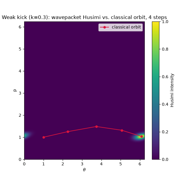
At weak kick strength the classical map is nearly integrable, and a narrow wavepacket’s Husimi peak tracks the corresponding classical orbit closely for a while, before quantum spreading and interference eventually take over – the correspondence principle in action, and its eventual breakdown.

k_weak = 0.3
qkr_weak = QuantumKickedRotor(k=k_weak, dim=500)
theta0, p0 = 1.0, 1.0
psi_weak = qkr_weak.coherent_state(theta0, p0)
n_steps = 4
states_weak = qkr_weak.evolve(psi_weak, n_steps=n_steps)
classical = StandardMap(k=k_weak).trajectory(np.array([theta0, p0]), n_iter=n_steps)

fig2, ax2 = plt.subplots(figsize=(6.5, 6))
q_grid, p_grid, husimi = qkr_weak.husimi(states_weak[-1], resolution=150)
plot_husimi(q_grid, p_grid, husimi, ax=ax2, q_label=r"$\theta$")
ax2.plot(classical[:, 0], classical[:, 1], "o-", color=theme.ACCENT, ms=5, label="classical orbit")
ax2.set_title(f"Weak kick (k={k_weak}): wavepacket Husimi vs. classical orbit, {n_steps} steps")
ax2.legend(loc="upper right")

plt.show()