The harmonic chain: normal modes, exactly

HarmonicChain models \(N\) identical point masses \(m\), connected in a line by identical springs of constant \(k\), with both ends clamped to fixed walls (\(q_0 = q_{N+1} = 0\)). Writing \(q_i\) and \(p_i\) for the displacement and momentum of mass \(i\), the system is the separable Hamiltonian

\[H = \sum_{i=1}^{N} \frac{p_i^2}{2m} + \frac{k}{2}\sum_{i=0}^{N} (q_{i+1} - q_i)^2 ,\]

whose equations of motion, \(m\ddot q_i = k(q_{i+1} - 2q_i + q_{i-1})\), are exactly linear and hence exactly solvable. The normal modes are the discrete sine waves

\[Q_k = \sqrt{\frac{2}{N+1}} \sum_{i=1}^{N} q_i \sin\!\left(\frac{i k \pi}{N+1}\right), \qquad \omega_k = 2\sqrt{\frac{k}{m}} \sin\!\left(\frac{k\pi}{2(N+1)}\right), \qquad k = 1, \dots, N,\]

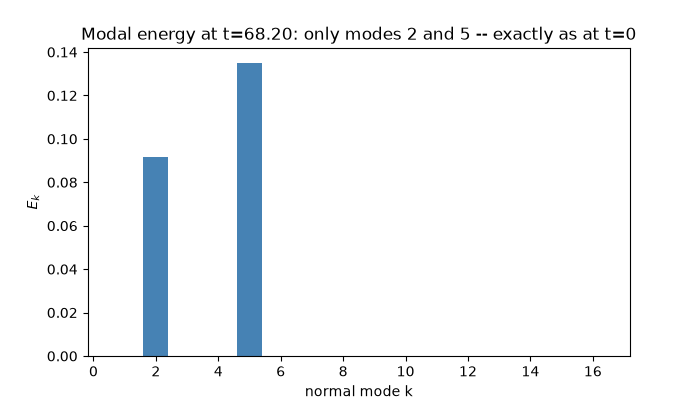
with modal energy \(E_k = \tfrac12 P_k^2/m + \tfrac12 m\omega_k^2 Q_k^2\). Because the system is exactly linear, each mode’s energy \(E_k\) is a separate constant of motion – excited modes never exchange energy. This exactly-solvable lattice is the reference point for the non-linear FPUTChain’s modal analysis (see The Fermi-Pasta-Ulam-Tsingou recurrence): here, exciting two modes (2 and 5) at once shows their energies stay exactly separate and constant forever – no mixing at all, in a linear system.

import matplotlib.pyplot as plt
import numpy as np

from physicskit.classical.systems.chains import HarmonicChain

n = 16
chain0 = HarmonicChain(np.zeros(n), np.zeros(n), k=1.0)
omegas = chain0.normal_mode_frequencies()

# Excite modes 2 and 5 simultaneously with independent amplitudes.
sites = np.arange(1, n + 1)
q0 = 0.4 * np.sin(sites * 2 * np.pi / (n + 1)) + 0.2 * np.sin(sites * 5 * np.pi / (n + 1))
chain = HarmonicChain(q0, np.zeros(n), k=1.0)

t_final = 4 * (2 * np.pi / omegas[1])  # a few periods of the slowest excited mode
result = chain.integrate((0, t_final), dt=0.01, method="yoshida4")

modal_history = np.array([chain.modal_energies(q, p) for q, p in zip(result.q[::20], result.p[::20])])
t_sampled = result.t[::20]

drift = np.max(np.abs(result.energy - result.energy[0])) / abs(result.energy[0])
print(f"relative energy drift: {drift:.3e}")
print(f"mode 2 energy range: [{modal_history[:, 1].min():.4f}, {modal_history[:, 1].max():.4f}]")
print(f"mode 5 energy range: [{modal_history[:, 4].min():.4f}, {modal_history[:, 4].max():.4f}]")

relative energy drift: 2.917e-10
mode 2 energy range: [0.0918, 0.0918]
mode 5 energy range: [0.1351, 0.1351]

Real-space motion: a beat pattern from two pure tones

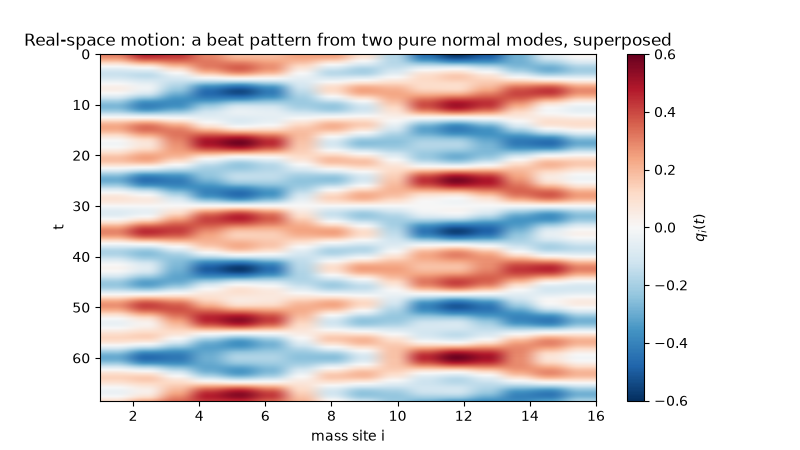
A flat line of “mode k energy vs t” alone is hard to read as physics; the spacetime picture of the displacement q_i(t) is what makes the underlying two-frequency beating (mode 2 + mode 5, superposed) visible directly.

fig1, ax = plt.subplots(figsize=(8, 4.5))
extent = [1, n, result.t[-1], result.t[0]]
im = ax.imshow(result.q[::5], aspect="auto", extent=extent, cmap="RdBu_r", vmin=-0.6, vmax=0.6)
ax.set_xlabel("mass site i")
ax.set_ylabel("t")
ax.set_title("Real-space motion: a beat pattern from two pure normal modes, superposed")
fig1.colorbar(im, ax=ax, label=r"$q_i(t)$")

fig2, ax2 = plt.subplots(figsize=(7, 4))
ax2.bar(np.arange(1, n + 1), modal_history[-1], color="steelblue")
ax2.set_xlabel("normal mode k")
ax2.set_ylabel(r"$E_k$")
ax2.set_title(f"Modal energy at t={t_sampled[-1]:.2f}: only modes 2 and 5 -- exactly as at t=0")

plt.show()

• 
•