
Note
Go to the end to download the full example code.
The Fermi-Pasta-Ulam-Tsingou recurrence#
FPUTChain is the classic
Fermi-Pasta-Ulam-Tsingou \(\beta\)-lattice: \(N\) fixed-end
masses \(m\) coupled by springs with an added quartic
non-linearity, so the inter-site stretch \(r_i = q_{i+1} - q_i\)
costs potential energy
giving the equation of motion \(m\ddot q_i = k(q_{i+1} - 2q_i +
q_{i-1}) + \beta\!\left[(q_{i+1}-q_i)^3 - (q_i - q_{i-1})^3\right]\).
Here a single low-order normal mode (mode 1) is excited initially, with
\(\beta = 1\). Fermi, Pasta, Ulam, and Tsingou expected the
non-linear coupling to thermalize the system – energy spreading evenly
across all normal-mode energies \(E_k\) (see
HarmonicChain,
The harmonic chain: normal modes, exactly, for the linear-mode decomposition).
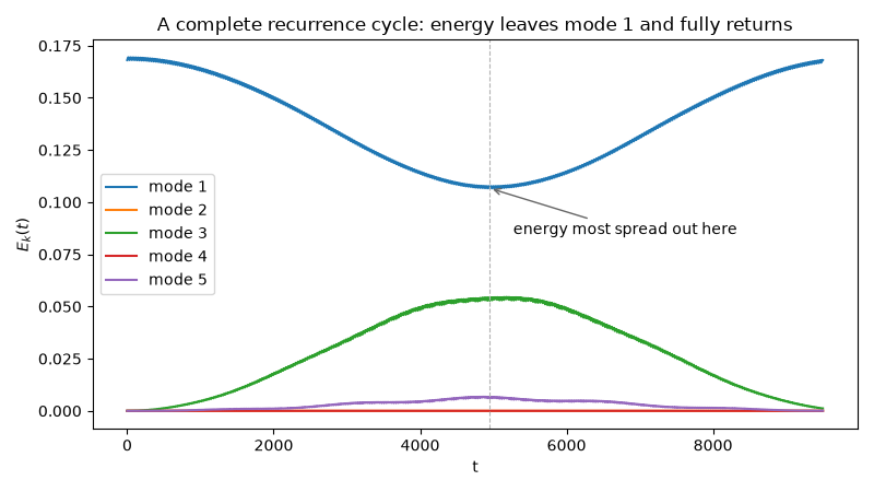
Instead the system shows the famous near-exact recurrence: energy
drains out of mode 1 into a couple of other low modes (mostly mode 3,
here) and then flows back, essentially returning to the original
single-mode state – a complete cycle, not thermalization. Contrast
this with HarmonicChain’s
perfectly rigid mode-separation (\(\beta = 0\), see
The harmonic chain: normal modes, exactly): the non-linearity is what lets modes
exchange energy at all, but not ergodically.
import matplotlib.pyplot as plt
import numpy as np

from physicskit.classical.systems.chains import FPUTChain
from physicskit.classical.visualizers.modal_analysis import plot_modal_energy_bars

chain = FPUTChain(n=32, beta=1.0, mode=1, amplitude=1.5)
e0 = chain.energy()
result = chain.integrate((0, 9500), dt=0.02, method="yoshida4")
drift = abs(result.energy[-1] - e0) / abs(e0)
print(f"relative energy drift over the full run: {drift:.3e}")

modal_history = np.array([chain.modal_energies(q, p) for q, p in zip(result.q[::200], result.p[::200])])
t_sampled = result.t[::200]
mode1_fraction = modal_history[:, 0] / e0
midpoint_idx = int(np.argmin(mode1_fraction))
print(
    f"mode-1 energy fraction: starts at {mode1_fraction[0]:.3f}, "
    f"dips to {mode1_fraction[midpoint_idx]:.3f} at t={t_sampled[midpoint_idx]:.0f}, "
    f"ends at {mode1_fraction[-1]:.3f}"
)

fig1, ax = plt.subplots(figsize=(8, 4.5))
for k in range(5):
    ax.plot(t_sampled, modal_history[:, k], label=f"mode {k + 1}")
ax.axvline(t_sampled[midpoint_idx], color="0.7", lw=0.8, ls="--")
annotate_xy = (t_sampled[midpoint_idx], modal_history[midpoint_idx, 0])
ax.annotate("energy most spread out here", xy=annotate_xy, xytext=(0.55, 0.5), textcoords="axes fraction", arrowprops=dict(arrowstyle="->", color="0.4"))
ax.set_xlabel("t")
ax.set_ylabel(r"$E_k(t)$")
ax.set_title("A complete recurrence cycle: energy leaves mode 1 and fully returns")
ax.legend()
fig1.tight_layout()
relative energy drift over the full run: 1.549e-12
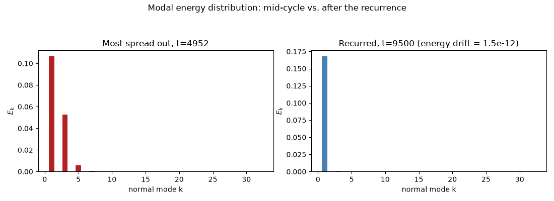
mode-1 energy fraction: starts at 0.992, dips to 0.630 at t=4952, ends at 0.992
Modal energy distribution: mid-cycle vs. after the recurrence#
fig2, axes2 = plt.subplots(1, 2, figsize=(11, 4))
plot_modal_energy_bars(chain, result.q[::200][midpoint_idx], result.p[::200][midpoint_idx], ax=axes2[0], color="firebrick")
axes2[0].set_title(f"Most spread out, t={t_sampled[midpoint_idx]:.0f}")
plot_modal_energy_bars(chain, result.q[-1], result.p[-1], ax=axes2[1], color="steelblue")
axes2[1].set_title(f"Recurred, t={result.t[-1]:.0f} (energy drift = {drift:.1e})")
fig2.suptitle("Modal energy distribution: mid-cycle vs. after the recurrence")
fig2.tight_layout(rect=[0, 0, 1, 0.92])

plt.show()
Check#
Fermi-Pasta-Ulam-Tsingou: instead of thermalizing, the energy leaves mode 1 and comes back almost entirely (recurrence), at conserved total energy.
assert drift < 1e-9
assert mode1_fraction[midpoint_idx] < 0.7 and mode1_fraction[-1] > 0.95
Total running time of the script: (0 minutes 3.258 seconds)