
Note
Go to the end to download the full example code.
Why symplectic integration: RK4 leaks energy, Yoshida4 does not#
All three integrators here advance the same eccentric two-body Kepler
orbit (KeplerSystem,
semi-major axis \(a=1\), eccentricity \(e=0.6\)), i.e. the same
Hamiltonian \(H(q,p)\) and the same Hamilton’s equations
\(\dot q = \partial H/\partial p,\ \dot p = -\partial H/\partial
q\); only the numerical scheme used to step them forward differs.
Velocity Verlet updates the separable \(H = T(p) + V(q)\) by
with \(F = -\partial V/\partial q\); Yoshida4 composes three such Verlet sub-steps with special coefficients to reach 4th-order accuracy. Both are symplectic maps – they exactly preserve phase-space volume – and it is exactly this qualitative property that this example is about: this is the single most important comparison in physicskit.classical. RK4 (a classical, non-symplectic integrator) looks fine over a short integration, but its energy error grows monotonically over a long one – here, a clean, almost perfectly linear drift of several percent over a few thousand time units. Verlet (2nd-order symplectic) and Yoshida4 (4th-order symplectic) instead keep the energy error bounded: it oscillates within a fixed band that never grows, no matter how long you integrate – Yoshida4’s band is additionally far tighter, since it is a higher-order method. This qualitative difference (bounded oscillation vs. unbounded drift), not just “smaller numbers,” is the actual reason physicskit.classical defaults every conservative system to a symplectic backend.
import matplotlib.pyplot as plt
import numpy as np

from physicskit.classical.systems.newtonian import KeplerSystem

dt = 0.05
t_final = 4000
methods = [
    ("rk4", "firebrick", "RK4 (non-symplectic)"),
    ("verlet", "orange", "Verlet (2nd-order symplectic)"),
    ("yoshida4", "steelblue", "Yoshida4 (4th-order symplectic)"),
]

results = {}
for method, _color, label in methods:
    system = KeplerSystem.from_orbital_elements(a=1.0, e=0.6)
    e0 = system.energy()
    result = system.integrate((0, t_final), dt=dt, method=method)
    drift = (result.energy - e0) / abs(e0)
    results[method] = (result.t, drift)
    print(f"{label}: final relative drift = {drift[-1]:+.4f}, max |drift| = {np.max(np.abs(drift)):.4f}")

fig, axes = plt.subplots(1, 2, figsize=(11, 4.5))
for method, color, label in methods:
    t, drift = results[method]
    axes[0].plot(t, drift, color=color, label=label, lw=1.2)
axes[0].set_xlabel("t")
axes[0].set_ylabel(r"$(H(t)-H(0))/H(0)$")
axes[0].set_title("RK4 drifts monotonically; symplectic methods stay bounded")
axes[0].legend(fontsize=9)

# Zoom in on just the two symplectic methods to see their bounded-oscillation
# structure, invisible at the scale RK4's drift forces on the left panel.
for method, color, label in methods[1:]:
    t, drift = results[method]
    axes[1].plot(t, drift, color=color, label=label, lw=1.0)
axes[1].set_xlabel("t")
axes[1].set_ylabel(r"$(H(t)-H(0))/H(0)$")
axes[1].set_title("Zoomed in: both symplectic methods, no RK4")
axes[1].legend(fontsize=9)
fig.tight_layout()

plt.show()
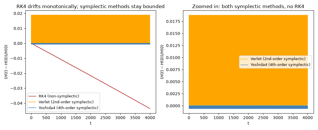
RK4 (non-symplectic): final relative drift = -0.0436, max |drift| = 0.0436
Verlet (2nd-order symplectic): final relative drift = +0.0181, max |drift| = 0.0188
Yoshida4 (4th-order symplectic): final relative drift = -0.0006, max |drift| = 0.0006
Check#
RK4’s energy error drifts in one direction; Verlet’s and Yoshida4’s stay bounded (Yoshida4 two orders of magnitude smaller), however long the run.
Total running time of the script: (0 minutes 1.682 seconds)