Automated timestep selection with estimate_dt

None of physicskit.classical’s integrators are adaptive: each takes a fixed step \(\Delta t\) for the whole run, so choosing \(\Delta t\) is normally a manual “integrate, check drift, halve or double, repeat” search – exactly what estimate_dt() automates, by searching for the largest \(\Delta t\) whose relative energy drift \(|H(t) - H(0)| / |H(0)|\) stays below a given tolerance over the full run. This runs it on two very different conservative systems: a quasi-periodic Kepler orbit (KeplerSystem, semi-major axis \(a=1\), eccentricity \(e=0.5\), governed by the inverse-square gravitational Hamiltonian), where a short probe already predicts the right \(\Delta t\), and a chaotic double pendulum (DoublePendulum, governed by its coupled Euler-Lagrange equations), where estimate_dt()’s own verification stage has to catch and shrink a fast-probe estimate that would otherwise fail once actually run for the full step count.

import matplotlib.pyplot as plt
import numpy as np

from physicskit.classical.systems.lagrangian import DoublePendulum
from physicskit.classical.systems.newtonian import KeplerSystem
from physicskit.classical.utils.stepsize import estimate_dt

A quasi-periodic system (Kepler orbit)

print("Quasi-periodic system (Kepler orbit):")
est_kepler = estimate_dt(
    lambda: KeplerSystem.from_orbital_elements(a=1.0, e=0.5),
    method="yoshida4",
    tol=1e-6,
    target_steps=100_000,
    probe_steps=2000,
    dt_initial=1e-2,
)
print(f"  dt = {est_kepler.dt:.4g}, achieved drift = {est_kepler.achieved_drift:.2e}, evaluations = {est_kepler.n_evaluations}")

Quasi-periodic system (Kepler orbit):
  dt = 0.01477, achieved drift = 9.92e-07, evaluations = 7

A chaotic system (double pendulum)

Found via bracket+bisect on a short probe, THEN verified – and if necessary shrunk further – at the full target_steps, which is what makes this safe for a chaotic system where a short probe alone can be misleading.

print("Chaotic system (double pendulum):")
est_dp = estimate_dt(
    lambda: DoublePendulum([2.0, 1.0], [0.5, -0.3]),
    method="implicit_midpoint",
    tol=1e-6,
    target_steps=100_000,
    probe_steps=2000,
    dt_initial=1e-3,
)
print(f"  dt = {est_dp.dt:.4g}, achieved drift = {est_dp.achieved_drift:.2e}, evaluations = {est_dp.n_evaluations}")

Chaotic system (double pendulum):
  dt = 3.716e-05, achieved drift = 4.14e-07, evaluations = 11

Making the search visible: a direct drift-vs-dt sweep

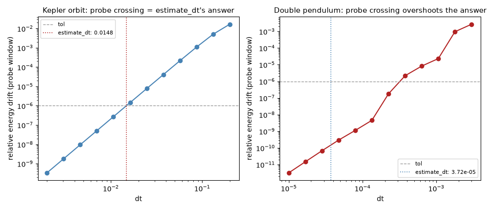
The prints above show only the two endpoints of the search – estimate_dt’s starting guess and its final, verified answer. A direct sweep over dt, all measured on the same short probe_steps window the fast bracket-and-bisect stage itself uses, draws the underlying drift-vs-dt curve each search is bisecting along – and makes the difference between the two systems concrete rather than just asserted. For the Kepler orbit, the probe-window curve crosses tol almost exactly at the dt estimate_dt actually returns: the short probe is trustworthy on its own. For the double pendulum, the probe-window curve only crosses tol at a dt several times larger than estimate_dt’s returned value – a fast probe alone would have picked a dt that looks fine over 2000 steps but fails once the chaotic trajectory is actually run out to the full target_steps, which is exactly why the verification-and-shrink stage exists.

def sweep_drift(system_factory, method, dts, n_steps):
    drifts = np.empty_like(dts)
    for i, dt in enumerate(dts):
        system = system_factory()
        e0 = system.energy()
        result = system.integrate((0.0, n_steps * dt), dt=dt, method=method)
        drifts[i] = np.max(np.abs(result.energy - e0)) / abs(e0)
    return drifts


probe_steps = 2000
dts_kepler = np.geomspace(2e-3, 0.2, 12)
drift_kepler = sweep_drift(lambda: KeplerSystem.from_orbital_elements(a=1.0, e=0.5), "yoshida4", dts_kepler, probe_steps)

dts_dp = np.geomspace(1e-5, 3e-3, 12)
drift_dp = sweep_drift(lambda: DoublePendulum([2.0, 1.0], [0.5, -0.3]), "implicit_midpoint", dts_dp, probe_steps)

fig, axes = plt.subplots(1, 2, figsize=(10, 4.3))
axes[0].loglog(dts_kepler, drift_kepler, "o-", color="steelblue")
axes[0].axhline(1e-6, color="0.6", ls="--", lw=1, label="tol")
axes[0].axvline(est_kepler.dt, color="firebrick", ls=":", lw=1.2, label=f"estimate_dt: {est_kepler.dt:.3g}")
axes[0].set_xlabel("dt")
axes[0].set_ylabel("relative energy drift (probe window)")
axes[0].set_title("Kepler orbit: probe crossing = estimate_dt's answer", fontsize=10.5)
axes[0].legend(fontsize=8)

axes[1].loglog(dts_dp, drift_dp, "o-", color="firebrick")
axes[1].axhline(1e-6, color="0.6", ls="--", lw=1, label="tol")
axes[1].axvline(est_dp.dt, color="steelblue", ls=":", lw=1.2, label=f"estimate_dt: {est_dp.dt:.3g}")
axes[1].set_xlabel("dt")
axes[1].set_ylabel("relative energy drift (probe window)")
axes[1].set_title("Double pendulum: probe crossing overshoots the answer", fontsize=10.5)
axes[1].legend(fontsize=8)
fig.tight_layout()

plt.show()