Maupertuis and Euler: the principle of least action

Maupertuis (1744) proposed that nature moves bodies so as to make an “action” as small as possible; Euler, the same year, put the idea on a mathematical footing. In Lagrange’s later form, the path a system takes between two fixed endpoints makes the action

\[S[x] = \int_0^T \left(\tfrac12 m\dot x^2 - V(x)\right) dt\]

stationary. This example finds the path directly, by discretizing \(S\) and minimizing it numerically over every interior point – no equation of motion is written down – and compares the result with the solution of Newton’s equation for a harmonic oscillator, \(x(t)=\sin\omega t/\sin\omega T\). It then shows the catch in the word least: for a long enough time interval, the true path is a saddle of \(S\), not a minimum.

import matplotlib.pyplot as plt
import numpy as np
from scipy.optimize import minimize

m, omega = 1.0, 1.0
x_start, x_end = 0.0, 1.0


def action(x_interior, T):
    """Discretized action with fixed endpoints (midpoint rule for V)."""
    x = np.concatenate([[x_start], x_interior, [x_end]])
    h = T / (len(x) - 1)
    kinetic = 0.5 * m * np.diff(x) ** 2 / h
    x_mid = 0.5 * (x[1:] + x[:-1])
    potential = 0.5 * m * omega**2 * x_mid**2 * h
    return np.sum(kinetic - potential)


def exact_path(t, T):
    return np.sin(omega * t) / np.sin(omega * T)

Minimizing the action finds the physical path

Start from a deliberately bad guess – a straight line plus noise – and let the optimizer lower \(S\). The minimizer lands on Newton’s solution to discretization accuracy.

N = 200
T = 2.0  # shorter than half a period, pi/omega
t = np.linspace(0.0, T, N + 1)
rng = np.random.default_rng(1744)
guess = np.linspace(x_start, x_end, N + 1)[1:-1] + 0.3 * rng.standard_normal(N - 1)
result = minimize(action, guess, args=(T,), method="L-BFGS-B", options={"maxiter": 20000, "maxfun": 10**6})
x_best = np.concatenate([[x_start], result.x, [x_end]])

print(f"S(initial guess) = {action(guess, T):.5f}")
print(f"S(minimizer)     = {result.fun:.5f}")
print(f"S(exact path)    = {action(exact_path(t, T)[1:-1], T):.5f}")
print(f"max |x_min - x_exact| = {np.max(np.abs(x_best - exact_path(t, T))):.2e}")

fig1, ax1 = plt.subplots(figsize=(5.5, 4))
ax1.plot(t, np.concatenate([[x_start], guess, [x_end]]), color="0.75", lw=0.8, label="starting guess")
ax1.plot(t, x_best, color="steelblue", lw=3, label="minimum of $S$")
ax1.plot(t, exact_path(t, T), "--", color="orange", label=r"$\sin\omega t/\sin\omega T$")
ax1.set_xlabel("t")
ax1.set_ylabel("x")
ax1.set_title("The path of stationary action")
ax1.legend(fontsize=8)
fig1.tight_layout()

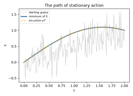
S(initial guess) = 1722.97544
S(minimizer)     = -0.22882
S(exact path)    = -0.22882
max |x_min - x_exact| = 7.62e-04

Least, or only stationary?

Perturb the true path by \(\epsilon\,\sin(\pi t/T)\), which keeps the endpoints fixed. For \(T<\pi/\omega\) every perturbation raises \(S\): a true minimum. Past the first kinetic focus, \(T>\pi/\omega\), this perturbation lowers \(S\) – the path is still stationary (the slope at \(\epsilon=0\) vanishes) but it is a saddle. Euler’s condition is stationarity; “least” was Maupertuis’s hopeful reading.

eps = np.linspace(-0.5, 0.5, 101)
fig2, ax2 = plt.subplots(figsize=(5.5, 4))
for T_i, color in [(2.0, "steelblue"), (4.0, "firebrick")]:
    t_i = np.linspace(0.0, T_i, N + 1)
    eta = np.sin(np.pi * t_i / T_i)
    S0 = action(exact_path(t_i, T_i)[1:-1], T_i)
    dS = np.array([action((exact_path(t_i, T_i) + e * eta)[1:-1], T_i) - S0 for e in eps])
    curvature = np.polyfit(eps, dS, 2)[0]
    kind = "minimum" if curvature > 0 else "saddle"
    print(f"T = {T_i} ({'<' if T_i < np.pi else '>'} pi): S(eps) - S(0) ~ {curvature:+.3f} eps^2  -> {kind}")
    ax2.plot(eps, dS, color=color, label=rf"$T={T_i}$ ({kind})")
ax2.axhline(0, color="0.7", lw=0.8)
ax2.set_xlabel(r"perturbation size $\epsilon$")
ax2.set_ylabel(r"$S[x+\epsilon\eta]-S[x]$")
ax2.set_title("Stationary, but not always least")
ax2.legend(fontsize=8)
fig2.tight_layout()

plt.show()

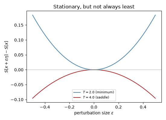
T = 2.0 (< pi): S(eps) - S(0) ~ +0.734 eps^2  -> minimum
T = 4.0 (> pi): S(eps) - S(0) ~ -0.383 eps^2  -> saddle

Check

Minimizing the discretized action recovers x(t) = sin(wt)/sin(wT); along eta = sin(pi t / T) the second variation is (pi^2 / 4T - w^2 T / 4) eps^2: a minimum for T < pi/w, a saddle beyond.

assert abs(result.fun - action(exact_path(t, T)[1:-1], T)) < 1e-6
assert np.max(np.abs(x_best - exact_path(t, T))) < 2e-3
for T_i in (2.0, 4.0):
    t_i = np.linspace(0.0, T_i, N + 1)
    eta = np.sin(np.pi * t_i / T_i)
    S0 = action(exact_path(t_i, T_i)[1:-1], T_i)
    dS = np.array([action((exact_path(t_i, T_i) + e * eta)[1:-1], T_i) - S0 for e in eps])
    assert abs(np.polyfit(eps, dS, 2)[0] - (np.pi**2 / (4 * T_i) - omega**2 * T_i / 4)) < 1e-3