Kepler orbits and perihelion precession

KeplerSystem is the planar, reduced 2-body problem in the center-of-mass frame, a separable Hamiltonian in Cartesian coordinates \(q=(x,y)\), \(p=(p_x,p_y)\),

\[H(q, p) = \frac{|p|^2}{2\mu} + V(r), \qquad r = |q|, \qquad V(r) = -\frac{k}{r} + \frac{c_\mathrm{pn}}{r^3} ,\]

with \(k\) the gravitational coupling, \(\mu\) the reduced mass, and \(c_\mathrm{pn}\) an effective post-Newtonian correction that reproduces the qualitative apsidal (perihelion) precession General Relativity predicts for Mercury’s orbit. Both terms are purely radial, so the exactly conserved Laplace-Runge-Lenz vector of the pure Kepler problem,

\[\mathbf{A} = \mathbf{p} \times L - \mu k \hat{\mathbf{r}}, \qquad L = x p_y - y p_x ,\]

slowly precesses once \(c_\mathrm{pn} \neq 0\), even though the system remains conservative and separable. Shows a pure 1/r orbit’s closed ellipse next to the precessing rosette produced by the post-Newtonian correction, then verifies the key physical claim: total energy stays conserved (to machine precision, via Yoshida4) even as the Laplace-Runge-Lenz vector’s direction slowly rotates – the signature of apsidal precession, e.g. Mercury’s orbit.

import matplotlib.pyplot as plt
import numpy as np

from physicskit.classical.systems.newtonian import KeplerSystem
from physicskit.classical.utils.conservation import relative_energy_drift

Pure ellipse vs. precessing rosette

pure = KeplerSystem.from_orbital_elements(a=1.0, e=0.5)
perturbed = KeplerSystem.from_orbital_elements(a=1.0, e=0.5, c_pn=0.008)

res_pure = pure.integrate((0, 40), dt=1e-3, method="yoshida4")
res_pert = perturbed.integrate((0, 40), dt=1e-3, method="yoshida4")

fig1, axes = plt.subplots(1, 2, figsize=(9, 4.2))
axes[0].plot(res_pure.q[:, 0], res_pure.q[:, 1], color="steelblue", lw=0.8)
axes[0].plot(0, 0, "o", color="gold")
axes[0].set_title("Pure 1/r: closed ellipse")
axes[0].set_aspect("equal")

axes[1].plot(res_pert.q[:, 0], res_pert.q[:, 1], color="firebrick", lw=0.6)
axes[1].plot(0, 0, "o", color="gold")
axes[1].set_title("With c_pn: precessing rosette")
axes[1].set_aspect("equal")
fig1.tight_layout()

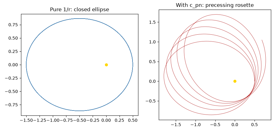
Energy stays flat while the LRL vector precesses

Both terms in V(r) are still purely radial (velocity-independent), so the system remains conservative and separable – Yoshida4 keeps the energy to machine precision even though the LRL vector itself is no longer a constant of motion.

system = KeplerSystem.from_orbital_elements(a=1.0, e=0.5, c_pn=0.008)
lrl0 = system.lrl_vector()
result = system.integrate((0, 200), dt=1e-3, method="yoshida4")

lrl_vecs = np.array([system.lrl_vector(q, p) for q, p in zip(result.q, result.p)])
angle = np.arctan2(lrl_vecs[:, 1], lrl_vecs[:, 0]) - np.arctan2(lrl0[1], lrl0[0])
drift = relative_energy_drift(result.energy)
print(f"total perihelion precession over t=200: {np.unwrap(angle)[-1]:.4f} rad")
print(f"max relative energy drift: {np.max(drift):.3e}")

fig2, axes2 = plt.subplots(1, 2, figsize=(9, 3.8))
axes2[0].plot(result.t, np.unwrap(angle), color="firebrick")
axes2[0].set_xlabel("t")
axes2[0].set_ylabel("LRL precession angle (rad)")
axes2[0].set_title("Perihelion advance")

axes2[1].semilogy(result.t, drift, color="steelblue")
axes2[1].set_xlabel("t")
axes2[1].set_ylabel("|H(t) - H(0)| / |H(0)|")
axes2[1].set_title("Energy still conserved")
fig2.tight_layout()

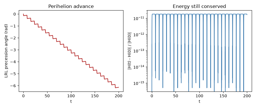
total perihelion precession over t=200: -6.1370 rad
max relative energy drift: 1.823e-11

This is the same physics as Free fall with an oblique velocity: the cannonball problem (a conservative central force integrated symplectically), generalized from uniform gravity to an inverse-square field with a relativistic correction.

plt.show()