The Foucault pendulum and Earth’s rotation

FoucaultPendulum models a small-oscillation pendulum’s horizontal displacement \(q=(x,y)\) (\(x\) = East, \(y\) = North) as seen from the rotating surface of the Earth. In a non-rotating (inertial) frame it would obey the isotropic harmonic equation \(\ddot q = -\omega_0^2 q\), \(\omega_0 = \sqrt{g/\ell}\); but Earth’s surface itself turns about the local vertical at rate \(\omega_z = \omega_\mathrm{earth}\sin(\text{latitude})\), adding a velocity-dependent Coriolis term:

\[\ddot x = -\omega_0^2 x + 2\omega_z \dot y, \qquad \ddot y = -\omega_0^2 y - 2\omega_z \dot x .\]

Leon Foucault’s 1851 pendulum at the Paris Pantheon proved Earth rotates without looking at the sky: viewed from the ground, this Coriolis term steadily precesses the pendulum’s swing plane at a rate set only by latitude, while total energy \(E = |v|^2/2 + \omega_0^2 |q|^2 / 2\) – untouched by a force that is always perpendicular to the velocity – stays exactly conserved. This example reproduces both the rosette trace on the ground and the “unwound” fixed-plane swing seen in the frame that co-rotates with the precession.

import matplotlib.pyplot as plt
import numpy as np

from physicskit.classical.systems.newtonian import FoucaultPendulum
from physicskit.classical.utils.conservation import relative_energy_drift

The rosette traced on the ground

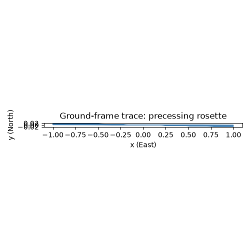
Released from rest at a fixed deflection, the pendulum’s tip does not retrace a single line: each swing’s plane is rotated slightly from the last, tracing out a rosette over one “Foucault day”.

system = FoucaultPendulum.from_deflection(amplitude=1.0, latitude_deg=48.85)  # Paris Pantheon
print(f"swing period: {2 * np.pi / system.omega0:.2f} s")
print(f"precession period (Foucault day): {system.precession_period() / 3600:.2f} hours")

result = system.integrate((0.0, 400.0), dt=1e-3, method="implicit_midpoint")
x, y = result.y[:, 0], result.y[:, 1]

fig1, ax1 = plt.subplots(figsize=(5, 5))
ax1.plot(x, y, lw=0.4, color="steelblue")
ax1.set_xlabel("x (East)")
ax1.set_ylabel("y (North)")
ax1.set_title("Ground-frame trace: precessing rosette")
ax1.set_aspect("equal")
fig1.tight_layout()

swing period: 16.42 s
precession period (Foucault day): 31.79 hours

Unwinding the precession

Rotating the trajectory by +omega_z * t undoes the precession: in this co-rotating frame the pendulum swings back and forth in a single fixed plane, exactly like an ordinary non-rotating pendulum – the frame from which Earth itself is seen to be turning underneath.

x_rot, y_rot = FoucaultPendulum.to_corotating_frame(x, y, result.t, system.omega_z)

fig2, ax2 = plt.subplots(figsize=(5, 5))
ax2.plot(x_rot, y_rot, lw=0.4, color="firebrick")
ax2.set_xlabel("x (co-rotating)")
ax2.set_ylabel("y (co-rotating)")
ax2.set_title("Co-rotating frame: a single fixed swing plane")
ax2.set_aspect("equal")
fig2.tight_layout()

Energy stays flat while the swing plane precesses

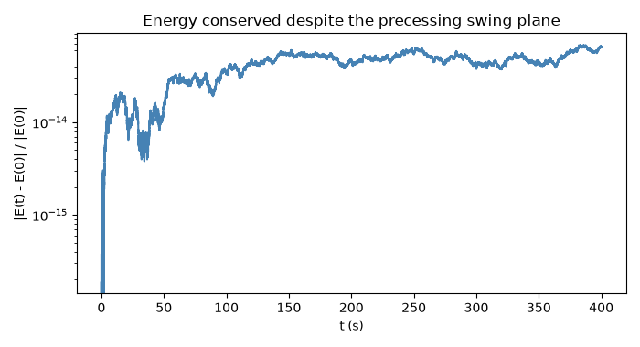
The Coriolis term does no work, so total mechanical energy is conserved to machine precision even though the swing plane itself rotates steadily – verified here against the closed-form small-oscillation solution.

x_analytic, y_analytic = FoucaultPendulum.analytic_solution([1.0, 0.0], [0.0, 0.0], system.omega0, system.omega_z, result.t)
drift = relative_energy_drift(result.energy)
print(f"max |x_numeric - x_analytic|: {np.max(np.abs(x - x_analytic)):.3e}")
print(f"max relative energy drift: {np.max(drift):.3e}")

fig3, ax3 = plt.subplots(figsize=(7, 3.8))
ax3.semilogy(result.t, drift, color="steelblue")
ax3.set_xlabel("t (s)")
ax3.set_ylabel("|E(t) - E(0)| / |E(0)|")
ax3.set_title("Energy conserved despite the precessing swing plane")
fig3.tight_layout()

plt.show()

max |x_numeric - x_analytic|: 1.859e-06
max relative energy drift: 6.824e-14